Originally posted on March 19, 2015 at Climate Etc.
A new paper on aerosol radiative forcing has important implications for estimates of climate sensitivity.
In a paper published last year (Lewis & Curry 2014), discussed here, Judith Curry and I derived best estimates for equilibrium/effective climate sensitivity (ECS) and transient climate response (TCR). At 1.64°C, our estimate for ECS was below all those exhibited by CMIP5 global climate models, and at 1.33°C for TCR, nearly all. However, our upper (95%) uncertainty bounds, at 4.05°C for ECS and 2.5°C for TCR, ruled out only a few CMIP5 climate models. The main reason was that they reflected the AR5 aerosol forcing best estimate and uncertainty range of −0.9 W/m2 (for 2011 vs 1750), with a 5–95% range of −1.9 to −0.1 W/m2. The strongly negative 5% bound of that aerosol forcing range accounts for the fairly high upper bounds on ECS and TCR estimates derived from AR5 forcing estimates.
The AR5 aerosol forcing best estimate and range reflect a compromise between satellite-instrumentation based estimates and estimates derived directly from global climate models. Although it is impracticable to estimate indirect aerosol forcing – that arising through aerosol-cloud interactions, which is particularly uncertain – without some involvement of climate models, observations can be used to constrain model estimates, with the resulting estimates generally being smaller and having narrower uncertainty ranges than those obtained directly from global climate models. Inverse estimates of aerosol forcing (derived by diagnosing the effects of aerosols on more easily estimated quantities, such as spatiotemporal surface temperature patterns) tended also to be smaller and less uncertain than those from climate models, but were disregarded in AR5.
Since AR5, various papers concerning aerosol forcing have been published, without really narrowing down the uncertainty range. Aerosol forcing is extremely complex, and estimating it is very difficult. One major problem is that indirect aerosol forcing has, approximately, a logarithmic relationship to aerosol levels. As a result, the change in aerosol forcing over the industrial period – anthropogenic aerosol forcing – is sensitive to the exact level of preindustrial aerosols (Carslaw et al 2013), and determining natural aerosol background levels is very difficult.
In this context, what is IMO a compelling new paper by Bjorn Stevens estimating aerosol forcing using multiple physically-based, observationally-constrained approaches is a game changer. Bjorn Stevens is Director of the Department ‘Atmosphere in the Earth System’ at the MPI for Meteorology in Hamburg. Stevens is an expert on cloud processes and their role in the general circulation and climate change. Through the introduction of new constraints arising from the time history of forcing and asymmetries in Earth’s energy budget, Stevens derives a lower limit for total aerosol forcing, from 1750 to recent years, of −1.0 W/m2. Although there is no best estimate given in the published paper, it can be worked out (from the uncertainty analyses given) to be −0.5 W/m2, and a time series for it derived from an analytical fit used in the analysis. An upper bound of −0.3 W/m2 is also given, but that comes from an earlier study (Murphy et al., 2009) rather than being a new estimate.
I have re-run the Lewis & Curry 2014 calculations using aerosol forcing estimates in line with the analysis in the Stevens paper (see Appendix) substituted for the AR5 estimates. I’ve accepted the Murphy et al (2009) upper bound of −0.3 W/m2 adopted by Stevens despite, IMO, the AR5 upper bound of −0.1 W/m2 being more consistent with the error distribution assumptions in his paper.
The Lewis & Curry 2014 energy budget study involves comparing, between a base and a final period, changes in global mean surface temperature (GMST) with changes in effective radiative forcing and – for ECS only – in the rate of ocean etc. climate system heat uptake. The preferred pairing was 1859–1882 with 1995–2011, the longest early and late periods free of significant volcanic activity. These periods are well matched for influence from internal variability and provide the largest change in forcing (and hence the narrowest uncertainty ranges). Neither the original Lewis & Curry 2014 ECS and TCR estimates nor the new estimates are significantly influenced by the low increase in surface warming this century.
Table 1 shows ECS and TCR estimates using the Stevens 2015 based aerosol forcing estimates, with for comparison the original estimates based on AR5 aerosol forcings. Estimates are shown for the preferred 1859–1882 base period to 1995–2011 final period combination, and also for a similarly well-matched 1930–1950 base period to 1995–2011 final period combination. That combination involves lower forcing and GMST increases and more heat uptake uncertainty, but probably better forcing and temperature data. Estimates from two AR5-vintage studies that used zonal temperature data to form their own inverse estimates of aerosol forcing are also shown.

Table 1: Best estimates are medians (50% probability points). Ranges (Ring et al: none given) and aerosol forcings are to the nearest 0.05°C. § Aldrin et al. aerosol forcing estimate is for 1750–2007 and based on replacing the AR4 aerosol forcing distribution used as the prior in the study, which significantly biased the inverse estimate, with the AR5 distribution. * With +0.1 W/m2 added to adjust for omitted black-carbon-on-snow forcing affecting the inverse estimate of aerosol forcing due to its similar fingerprint.
Compared with using the AR5 aerosol forcing estimates, the preferred ECS best estimate using an 1859–1882 base period reduces by 0.2°C to 1.45°C, with the TCR best estimate falling by 0.1°C to 1.21°C. More importantly, the upper 83% ECS bound comes down to 1.8°C and the 95% bound reduces dramatically – from 4.05°C to 2.2°C, below the ECS of all CMIP5 climate models except GISS-E2-R and inmcm4. Similarly, the upper 83% TCR bound falls to 1.45°C and the 95% bound is cut from 2.5°C to 1.65°C. Only a handful of CMIP5 models have TCRs below 1.65°C.
CMIP5 models with high TCRs are able to match the historical instrumental GMST record, or even warm less, mainly because most of them have highly negative aerosol forcing that until recently offset the bulk of greenhouse gas and other positive forcings. The mean aerosol forcing in CMIP5 models for which it has been diagnosed is about −1.2 W/m2 over 1850–2000, two and a half times Stevens’ best estimate.
The new ECS and TCR estimates, and the uncertainty associated with them, can also be presented in the form of probability density functions, as in Figures 1 and 2. The PDFs are skewed due principally to the dominant uncertainty, that in forcing, affecting the denominator of the fractions used to estimate ECS and TCR.
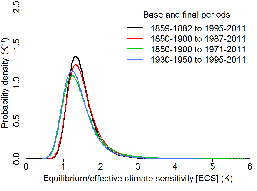
Figure 1: Energy budget estimated PDFs for ECS using Stevens 2015 based aerosol forcing
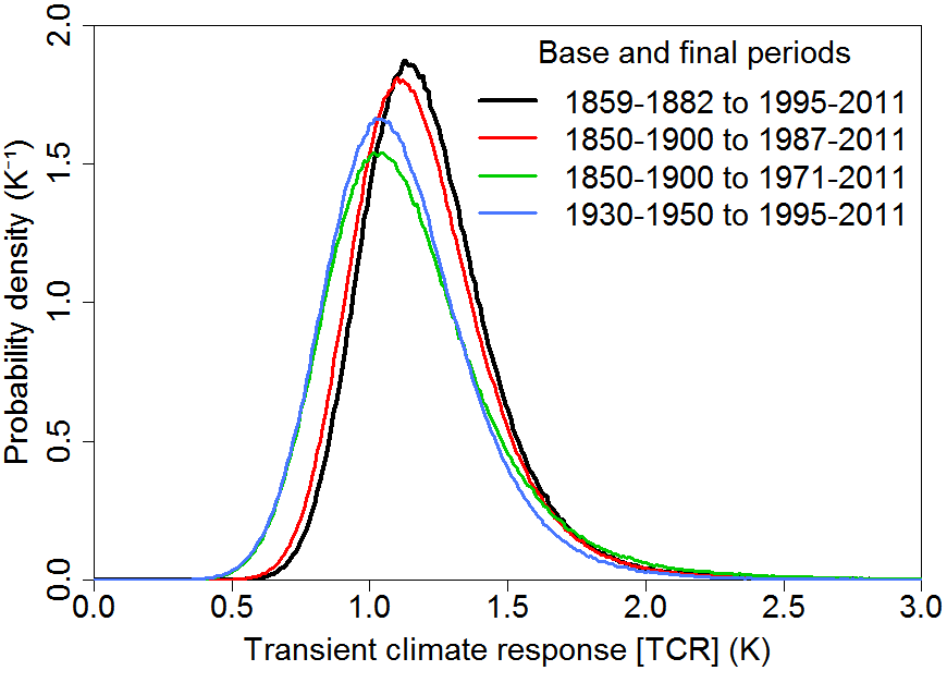
Figure 2: Energy budget estimated PDFs for TCR using Stevens 2015 based aerosol forcing
Appendix: Derivation of a best estimate time series for aerosol forcing from Stevens 2015
The best estimate for direct aerosol forcing (Fari) is taken as −0.15 W/m2 (line 494). The best estimate taken for indirect aerosol forcing (Faci) is that which, when δN/N has a bidirectional factor of two (0.5× to 2.0×) 5–95% uncertainty (line 620; taken as corresponding to a lognormal distribution) and C has a median estimate of 0.1 and a 95% bound of 0.15 (line 584; uncertainty independent and assumed Gaussian), produces a 95% bound for Faci of −0.75 W/m2. That implies a median estimate for Faci of −0.32 W/m2, which when added to the −0.15 W/m2 for Fari gives a best estimate for total aerosol forcing Faer of −0.5 W/m2.
The timeseries for Qa given by Eq.(A9) is used to scale, according to Eq.(1), the best estimate for Faer of −0.5 W/m2 as at 2005 over 1750 to 2011. Values of Qn = 76, α = 0.00167and β = 0.317 are used. Qn is taken from the caption to Fig.2 and α from the last line of Appendix A. The value of β is set to produce a total aerosol forcing of −0.5 W/m2 in 2005. Although giving a slightly different breakdown between Faci and Fari than that just derived, these parameter values result in an almost identical evolution of aerosol forcing.
Nicholas Lewis
References
Aldrin M, Holden M, Guttorp P, Skeie RB, Myhre G, Berntsen TK. Bayesian estimation of climate sensitivity based on a simple climate model fitted to observations of hemispheric temperatures and global ocean heat content. Environmetrics 23:253–271 (2012)
Carslaw, K. S., and coauthors. Large contribution of natural aerosols to uncertainty in indirect forcing. Nature, 503 (7474), 67–71 (2013)
Lewis N An objective Bayesian, improved approach for applying optimal fingerprint techniques to estimate climate sensitivity. J Clim 26:7414–7429 (2013)
Lewis N and Curry J A: The implications for climate sensitivity of AR5 forcing and heat uptake estimates, Climate Dynamics doi: 10.1007/s00382-014-2342-y (2014)
Stevens, B. Rethinking the lower bound on aerosol radiative forcing. In press, J.Clim (2015) doi: http://dx.doi.org/10.1175/JCLI-D-14-00656.1
Leave A Comment