Originally posted on July 5, 2011 at Climate Etc.
The IPCC Fourth Assessment Report of 2007 (AR4) contained various errors, including the well publicised overestimate of the speed at which Himalayan glaciers would melt. However, the IPCC’s defenders point out that such errors were inadvertent and inconsequential: they did not undermine the scientific basis of AR4. Here I demonstrate an error in the core scientific report (WGI) that came about through the IPCC’s alteration of a peer-reviewed result. This error is highly consequential, since it involves the only instrumental evidence that is climate-model independent cited by the IPCC as to the probability distribution of climate sensitivity, and it substantially increases the apparent risk of high warming from increases in CO2 concentration.
In the Working Group 1: The Physical Science Basis Report of AR4 (“AR4:WG1”), various studies deriving estimates of equilibrium climate sensitivity from observational data are cited, and a comparison of the results of many of these studies is shown in Figure 9.20, reproduced below. In most cases, probability density functions (PDFs) of climate sensitivity are given, truncated over the range of 0°C to 10°C and scaled to give a cumulative distribution function (CDF) of 1 at 10°C.
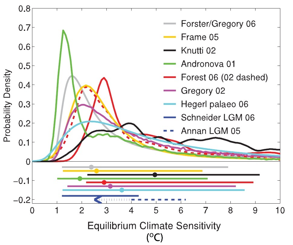
Figure 1. IPCC AR4:WG1 Figure 9.20. [Hegerl et al, 2007]
Of the eight studies for which PDFs are shown, only one – Forster/Gregory 06 [Forster and Gregory, 2006] – is based purely on observational evidence, with no dependence on any climate model simulations. Forster/Gregory 06 regressed changes in net radiative flux imbalance, less net radiative forcing, on changes in the global surface temperature, to obtain a direct measure of the overall climate response or feedback parameter (Y, units Wm-2 °C-1). This parameter is the increase in net outgoing radiative flux, adjusted for any change in forcings, for each 1°C rise in the Earth’s mean surface temperature. Forster/Gregory 06 then derived an estimate of equilibrium climate sensitivity (hereafter “climate sensitivity”, with value denoted by S), the rise in surface temperature for a doubling of CO2 concentration, using the generally accepted relation S = 3.7/Y °C.
Measuring radiative flux imbalances provides a direct measure of Y, and hence of S, unlike other ways of diagnosing climate sensitivity. The method is largely unaffected by unforced natural variability in surface temperature and uncertainties in ocean heat uptake, and is relatively insensitive to uncertainties in fairly slowly changing forcings such as tropospheric aerosols. The ordinary least squares (OLS) regression approach used will, however, underestimate Y in the presence of fluctuations in surface temperature that do not give rise to changes in net radiative flux fitting the linear model. Such fluctuations in surface temperature may well be caused by autonomous (non-feedback) variations in clouds, acting as a forcing but not modelled as such. The authors gave reasoned arguments for using OLS regression, stating additionally that – since OLS regression is liable to underestimate Y, and hence overestimate S – doing so reinforced the main conclusion of the paper, that climate sensitivity is relatively low.
Forster & Gregory found that their data gave a central estimate for Y of 2.3 ± 1.4 per °C, with a 95% confidence range. As they stated, this corresponds to S being between 1.0 and 4.1°C, with 95% certainty – what the IPCC calls ‘extremely likely’ – and a central (median) estimate for S of 1.6°C.
Forster & Gregory considered all relevant sources of uncertainty, and settled upon the standard assumption that errors in the observable parameters have a normal distribution. Almost all the uncertainty in fact arose from the statistical fitting of the regression line, with only a small contribution from uncertainties in radiative forcing measurements, and very little from errors in the temperature data. That supports use of OLS regression. The Forster/Gregory 06 results were obtained and presented in a form that accurately reflected the characteristics of the data, with error bands and details of error distribution assumptions, so permitting a valid PDF for S to be computed, and compared with the IPCC’s version.
It follows from Forster & Gregory’s method and error distribution assumption that the PDF of Y is symmetrical, and would be normal if a large number of observations existed. Strictly, the PDF of Y follows a t-distribution, which when the number of observations is limited has somewhat fatter tails than a normal distribution. But Forster & Gregory instead used a large number of random simulations to determine the likely uncertainty range, thereby robustly reflecting the actual distribution. The comparisons given below would in any case be much the same whether a t-distribution or a normal distribution were used. From the close match to the IPCC’s graph (see Figure 5, below) achieved using a normal error distribution, it is evident that the IPCC made a normality assumption, so that has also been done here. On that basis, Figure 2 shows what the PDF of Y looks like. The graph has been cut off at a lower limit of Y = 0.2, corresponding to the upper limit of S = 18.5 that the IPCC imposed when transforming the data, as explained below.
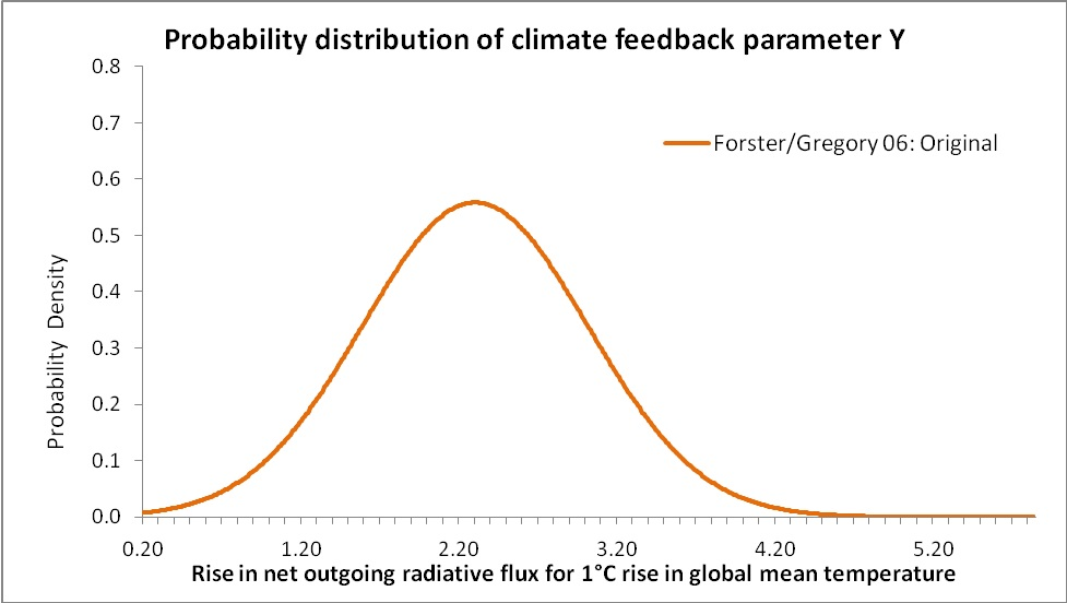
Figure 2
Knowing the PDF of Y, the PDF of the climate sensitivity S can readily be computed. It is shown in Figure 3. The x-axis is cut off at S = 10 to match Figure 1. The symmetrical PDF curve for Y gives rise to a very asymmetrical PDF curve for S, due to S having a reciprocal relationship with Y. The PDF shows that S is fairly tightly constrained, with S ‘extremely likely’ to lie in the range of 1.0–4.1°C and ‘likely’ (67% probability) to be between 1.2°C and 2.3°C.
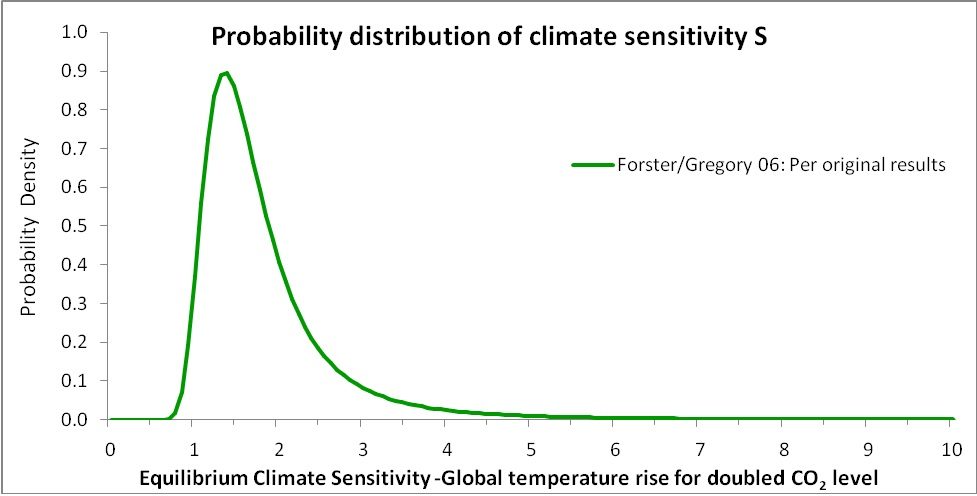
Figure 3
However, as Figure 4 below shows, the IPCC’s Forster/Gregory 06 PDF curve for S (as per Figure 1) is very different from the PDF based on the original results, shown in Figure 3. The IPCC curve is skewed substantially to higher climate sensitivities and has a much fatter tail than the original results curve. At the top of the ‘extremely likely’ range, it gives a 2.5% probability of the sensitivity exceeding 8.6°C, whereas the corresponding figure given in the original study is only 4.1°C. The top of the ‘likely’ range is doubled, from 2.3°C to 4.7°C, and the central (median) estimate is increased from 1.6°C to 2.3°C.
Figure 4
So what did the IPCC do to the original Forster/Gregory 06 results? The key lies in an innocuous sounding note in AR4:WG1concerning this study, below Figure 9.20: the IPCC have “transformed to a uniform prior distribution in ECS” (climate sensitivity), in the range 0–18.5°C. By using this prior distribution, the IPCC have imposed a starting assumption, before any data is gathered, that all climate sensitivities between 0°C and 18.5°C are equally likely, with other values ruled out. In doing so, the IPCC are taking a Bayesian statistical approach. Bayes’ theorem implies that the (posterior) probability distribution of an unknown parameter, in the light of data providing information on it, is given by multiplying a prior probability distribution thereof by the data-derived likelihood function[i], and then normalizing to give a unit CDF range.
Forster/Gregory 06 is not a Bayesian study – the form of the PDF for its estimate of Y, and hence for S, follows directly from the regression model used and error distribution assumptions made. It is possible to recast an OLS-regression, normal-error-distribution based study in Bayesian terms, but there is generally little point in doing so since the regression model and error distributions uniquely define the form of the prior distribution appropriate for a Bayesian interpretation. Indeed, Forster & Gregory stated that, since the uncertainties in radiative flux and forcing are proportionally much greater than those in temperature changes, their assumption that errors in these three variables are all normally distributed is approximately equivalent to assuming a uniform prior distribution in Y – implying (correctly) that to be the appropriate prior to use.
Returning to the PDFs concerned, can we be sure what exactly the IPCC actually did? Transforming the PDF for S to a uniform 0°C and 18.5°C prior distribution in S, and then truncating at 10°C as in Figure 1 (thereby making the 18.5°C upper limit irrelevant), is a simple enough mathematical operation to perform, on the basis that the original PDF effectively assumed a uniform prior in Y. At each value of S, one multiplies the original PDF value by S2, and then rescales so that the CDF is 1 at 10°C. On its own, doing this is not quite sufficient to make the original PDF for S match the IPCC’s version. It results in the dotted green line in Figure 5, which is slightly more peaked than the IPCC’s version, shown dashed in blue. It appears that the IPCC also increased the Forster/Gregory 06 uncertainty range for Y from ± 1.4 to ± 1.51, although there is no mention in AR4:WG1 of doing so. Making that change before transforming the original PDF to a uniform prior in S results in a curve, shown dotted in red in Figure 5, that emulates the IPCC’s version so closely that they are virtually indistinguishable.

Figure 5
Altering the probability density of S, by imposing a uniform prior distribution in S, also implicitly changes the probability density of Y, as the two parameters are directly (but inversely) related. The probability density of Y that equates to the IPCC’s Figure 9.20 PDF for Forster/Gregory 06 is shown as the pink line in Figure 6, below, with the observationally-derived original for comparison.

Figure 6
The IPCC’s implicit transformation has radically reshaped the observationally-derived PDF for Y, shifting the central estimate of 2.3 to below 1.5, and implying a vastly increased probability of Y being very low (and hence S very high).
Use of a uniform prior distribution with an infinite range is a device in Bayesian statistics intended to reflect a lack of knowledge, prior to information from actual measurement data, and any other information, being incorporated. Such a prior distribution is intended to be used on the basis that it is uninformative and will influence the final probability density little, if at all. And, when used appropriately (here, applied to Y rather than to S), that can indeed be the effect of a very wide, symmetrical uniform prior.
But the IPCC’s use of a uniform prior in S has a quite different effect. A uniform prior distribution in S effectively conveys a strong belief that S is high, and Y low. Far from being an uninformative prior distribution, a uniform distribution in S has a powerful effect on the final PDF – greatly increasing the probability of S being high relative to that of S being low – even when, as here, the measurement data itself provides a relatively well constrained estimate of S. That is due to the shape of the prior, not to the imposition of upper and lower bounds[ii] on S – or, equivalently, on Y. Since the likelihood function is very small at the chosen bounds, they have little effect.
What the ‘uniform prior distribution in S’ transformation effected by the IPCC does is scale the objectively determined probability densities at each value of Y, and at the corresponding reciprocal value of S, by the square of the particular value of S involved. Mathematically, the transformation is equivalent to imposing a prior probability distribution on Y that has the form 1/Y2. So, the possibility of the value of S being around 10 (and therefore Y being 0.37) is given 100 times the weight, relative to its true probability on the basis of a uniform prior in Y, of the possibility of the value of S being around 1 (and therefore Y being 3.7).
The IPCC did not attempt, in the relevant part of AR4:WG1 (Chapter 9), any justification from statistical theory, or quote authority for, restating the results of Forster/Gregory 06 on the basis of a uniform prior in S. Nor did the IPCC challenge the Forster/Gregory 06 regression model, analysis of uncertainties or error assumptions. The IPCC simply relied on statements [Frame et al. 2005] that ‘advocate’ – without any justification from statistical theory – sampling a flat prior distribution in whatever is the target of the estimate – in this case, S. In fact, even Frame did not advocate use of a prior uniform distribution in S in a case like Forster/Gregory 06. Nevertheless, the IPCC concluded its discussion of the issue by simply stating that “uniform prior distributions for the target of the estimate [the climate sensitivity S] are used unless otherwise specified”.
The transformation effected by the IPCC, by recasting Forster/Gregory 06 in Bayesian terms and then restating its results using a prior distribution that is inconsistent with the regression model and error distributions used in the study, appears unjustifiable. In the circumstances, the transformed climate sensitivity PDF for Forster/Gregory 06 in the IPCC’s Figure 9.20 can only be seen as distorted and misleading.
The foregoing analysis demonstrates that the PDF for Forster/Gregory 06 in the IPCC’s Figure 9.20 is invalid. But the underlying issue, that Bayesian use of a uniform prior in S conveys a strong belief in climate sensitivity being high, prejudging the observational evidence, applies to almost all of the Figure 9.20 PDFs.
[i] The likelihood function represents, as a function of the parameter involved, the relative probability of the actual observational data being obtained. The prior distribution may represent lack of knowledge as to the value of the parameter, with a view to the posterior PDF reflecting only the information provided by the data. Alternatively, it may represent independent knowledge about the probability distribution parameter that the investigator wishes to incorporate in the analysis and to be reflected in the posterior PDF.
[ii] There is logic in imposing bounds: as Y approaches zero climate sensitivity tends to infinity, and S becomes negative (implying an unstable climate system) if Y is less than zero. This situation is unphysical: the relative stability of the climate system over a long period puts some upper bound on S – and hence a lower bound on Y. Similarly, physical considerations imply some upper bound on Y, and hence a lower bound on S. The actual bounds chosen make little difference, provided the observationally-derived likelihood function has by then become very low. The appropriate form of the prior distribution for the Bayesian analysis is more obvious if the bounds are thought of as applying to the likelihood function, rather than to the prior. Equivalently, the bounds may be viewed as giving rise to a separate, uniform but bounded, likelihood function representing independent information, by which the posterior PDF resulting from an unbounded prior is multiplied in a second Bayesian step.