Originally a guest post November 17, 2018 at Climate Etc.
Introduction
The Resplandy et al. (2018) ocean heat uptake study (henceforth Resplandy18) is based on measured changes in the O2/N2 ratio of air sampled each year, compared to air stored in high pressure tanks originally sampled in the late 1980s and early 1990s, and in atmospheric CO2 concentration. These are combined to produce an estimate (ΔAPOObs) of changes in atmospheric potential oxygen since 1991 (ΔAPO). They break this series down into four components, including one attributable to ocean warming (ΔAPOClimate). By estimating the other three, they isolate the implied ΔAPOClimate and use it to estimate the change in ocean heat content. In two recent articles, here and here, I set out why I thought the trend in ΔAPOClimate – from which they derived their ocean heat uptake estimate – was overstated, and its uncertainty greatly understated.
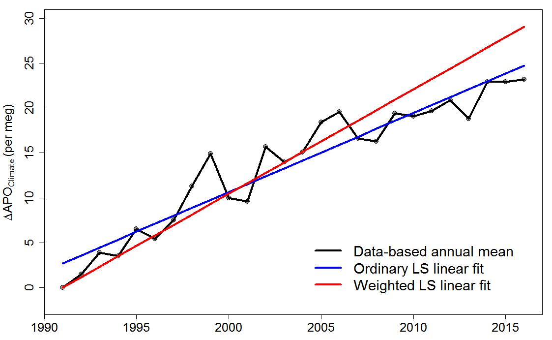
The easiest issue to explain is that they did not do a simple linear ordinary least squares regression through their ΔAPOClimate series, instead they used a weighted least squares regression with the weights taken from the 1σ (1 standard deviation) uncertainty estimates accompanying the data series. This was not made clear in the paper. Since they set the uncertainty to zero in 1991 by assumption, this effectively placed unlimited weight on the first observation, forcing the trend line through it and biasing the slope upwards, as shown in Figure 1 below.

Figure 1. Ordinary and weighted least squares regression linear fits to the ΔAPOClimate values.
In addition they did not calculate their uncertainties following the methods stated in their paper. Associated with ΔAPOObs and each of the components is a 1σ estimate that is intended to summarize its uncertainty range. One source of uncertainty in ΔAPOObs is thermal fractionation error (TFr) which arises because of temperature variations in the air storage tanks. Others include corrosion and leakage from tanks. Non-ΔAPOClimate components of ΔAPOObs also have uncertainties, including about biophysical processes and fossil fuel characteristics.
It turns out that TFr is the only significant component of the error in ΔAPOClimate that varies randomly in each year. Resplandy18 states that this error (1σ) is ± 2 per meg annually after July 1992, and ± 4 before. I therefore treat the TFr error for 1992 by splitting it into two halves, with these TFr errors assumed independent. How TFr errors were treated in Resplandy18 is unclear; it looks as if they were not reduced from ± 4 to ± 2 until the start of 1994.
As I will explain below, the other components of the uncertainty in ΔAPOClimate simply add up to a linear function of time, with a slight contribution proportional to the magnitude of the ΔAPOClimate series itself. Since ΔAPO values represent changes since 1991, by construction the error bounds for these components are zero in 1991 and scale up with time over 1992–2016. I recalculated the uncertainties using the source data described in Resplandy18 and I found them to be much larger than stated in the paper.
The second author on the paper, Ralph Keeling, has put out this statement:
I am working with my co-authors to address two problems that came to our attention since publication. These problems, related to incorrectly treating systematic errors in the O2 measurements and the use of a constant land O2:C exchange ratio of 1.1, do not invalidate the study’s methodology or the new insights into ocean biogeochemistry on which it is based. We expect the combined effect of these two corrections to have a small impact on our calculations of overall heat uptake, but with larger margins of error. We are redoing the calculations and preparing author corrections for submission to Nature.
He has also made a posting at realclimate.org describing the corrections they are proposing. I will comment on these below.
In this third article I show what I consider to be a correct estimation of the errors in ΔAPOClimate, of the trend in ΔAPOClimate, and of the uncertainty in that trend estimate, and I will incorporate the revised land O2:C exchange ratio that the authors now plan to use.
The nature of errors in ΔAPOClimate
Resplandy18 conducted a sensitivity analysis by generating a million sets of random number series scaled to have variances matching each of the measurement etc. error uncertainty ranges, recomputing the ΔAPOClimate values each time, then using the standard deviation of the resulting million values as the 1σ uncertainty for ΔAPOClimate.
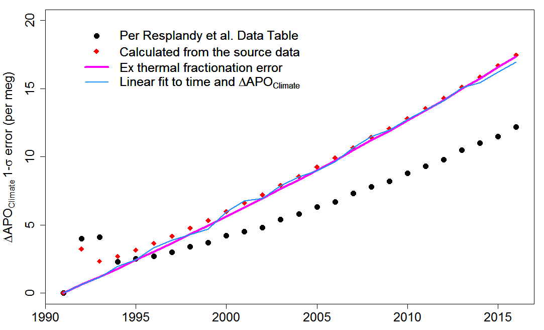
I have recalculated uncertainty in ΔAPOClimate using information from Resplandy18 Methods sections and Extended Data Table 3 and their relevant cited source studies. In Figure 2 I compare my estimates of how the total 1σ error magnitude develops over 1991–2016 (red diamonds) with the Resplandy18 Extended Data Table 4 values (black circles). I have adopted for the present their convention that there is zero TFr error in 1991.
Figure 2: Total 1σ error in ΔAPOClimate, for each year from 1991 to 2016, according to Resplandy18 and as calculated from source data. The magenta line shows how the size of total error develops when the thermal fractionation error element is excluded. The blue line shows that the development of {total error excluding thermal fractionation error} can be closely modelled by a fitted linear function of time since 1991 and magnitude of ΔAPOClimate.
After 1993, my calculated 1σ error magnitude exceeds that per Resplandy18. When the random annual TFr error is removed, my calculated remaining error 1σ magnitude (magenta line in Figure 1) grows almost linearly with elapsed years (year − 1991). It can be modelled as 0.667 ´ Elapsed years with a R2 of 0.999.
This almost perfect fit arises because the non-TFr error consists primarily of trend uncertainty (components that rise linearly over time) plus a lesser amount of scale uncertainty (components that rise linearly with the ΔAPO values themselves), with the small remainder relating mainly to fossil fuel emissions uncertainty, the annual errors in which are highly autocorrelated.[1] Trend errors in ΔAPOClimate increase linearly with time, emissions uncertainties almost do so, while scale-systematic errors increase linearly with ΔAPOClimate – which to a first approximation itself increases linearly with time. The non-TFr error 1σ can be modelled even more accurately as a linear function of both time and ΔAPOClimate (thin blue line in Figure 2), with an R2 of 0.9996.
It is not only the 1σ magnitude of the non-TFr errors – their standard deviation – but the actual errors in each year that can be accurately modelled as a function of time. When I sample randomly all the non-TFr error contributions to the ΔAPOClimate time series and model those errors as a multiple of elapsed years, the median R2 is 0.991, rising to 0.995 if ΔAPOClimate is also used as an explanatory variable. That is because the non-TFr errors have no randomness for individual years. Each component of them depends on a parameter that is determined once, randomly, with that value applying throughout the 1991–2016 period.
The inapplicability of Resplandy18’s statistical model
A simple linear trend regression is based the assumption that the dependant variables yt are affected by independent, random errors εt with zero mean. That is:
yt = a +bt + εt with all the εt independent
If the errors εt are independent and all have equal variance, ordinary least squares (OLS) regression is optimal for estimating the trend b. If the variances are not constant (which is called heteroscedasticity) then weighted least squares (WLS), in which the weight given to the squared error for each data point t is inversely proportional to the variance of εt, is optimal.[2] If the function being fitted can accurately represent the expected value of the variable y, both OLS and WLS will produce unbiased estimates of the function parameters – of the intercept and slope, in the case of a linear function – but with WLS providing a more precise (smaller uncertainty) estimate if the εt have unequal variances.
It appears that Resplandy18 used WLS regression on the ΔAPOClimate time series to estimate its trend. However, there is a problem with doing so here. While the ΔAPOClimate uncertainty estimates vary over time, the diagnosis of heteroscedasticity is correctly based not on those uncertainties but on the regression residuals. Their regression residuals are not heteroscedastic.[3] Neither are the residuals serially-dependent.[4]
Consequently OLS is the appropriate method to use and the trend estimate is 0.88 per meg per year, being the slope of the OLS linear fit in Figure 1. It can be seen that the WLS fit, which has a slope of 1.16 per meg per year, considerably overestimates ΔAPOClimate values in later years.
A quadratic trend?
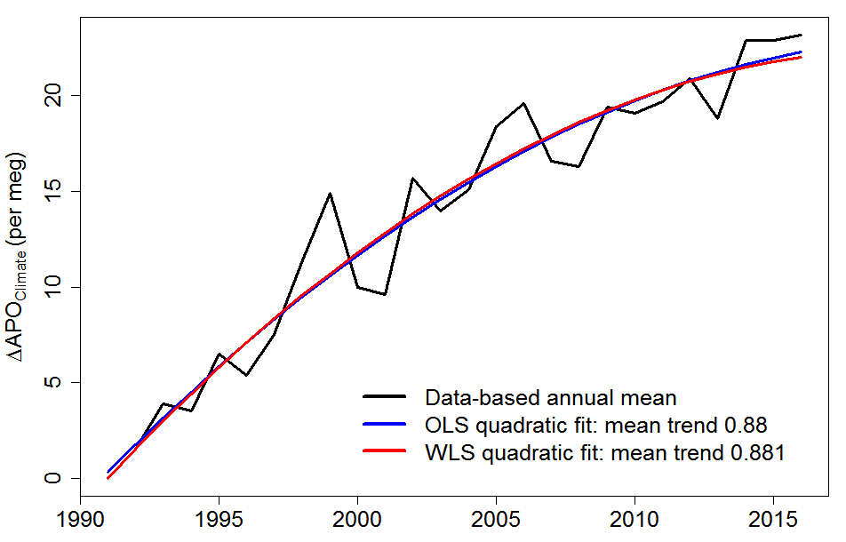
It can be seen from Figure 1 that a linear fit to ΔAPOClimate is not particularly good. The bias in direct WLS estimation of the trend in ΔAPOClimate arises from the combination of the flawed statistical error model with a linear function not being able to model ΔAPOClimate accurately. By forcing the WLS linear trend to go through the 1991 value the slope is biased upward. However, OLS estimation shows that a squared time trend variable belongs in the model (p = 0.002) and when it is included the fitted quadratic line goes almost exactly through the 1991 value. This neutralizes the WLS bias associated with the assumption of zero uncertainty in 1991. Figure 3 shows that WLS applied to estimate a quadratic trend yields a nearly identical fit to OLS, primarily because the constraint on the first observation now has little influence. The estimated mean trend over 1991–2016 is nearly identical in both cases (OLS +0.880 per year, WLS +0.881 per year).
Figure 3. Ordinary and weighted least squares regression quadratic fits to the ΔAPOClimate values.
Estimating the uncertainty in the ΔAPOClimate trend estimate
Since most of the measurement uncertainty in ΔAPOClimate is characterized by Resplandy18 as a linear trend it can be removed (or reduced to a constant term) by taking the first differences:
dAPOClimate = ΔAPOClimate[1992:2016] − ΔAPOClimate[1991:2015]
Note that the mean of dAPOClimate (0.93) corresponds to the trend in ΔAPOClimate,, and a regression of dAPOClimate on a constant and a trend would correspond to a quadratic trend estimation. Although taking first differences removes the linearly-trending portion of the uncertainties in different years that exists in the ΔAPOClimate time series, the first difference uncertainties still contain a component that does not vary randomly from year to year. While that component is not fast growing, it dominates uncertainty in trend estimation since, unlike the random annual TFr errors, its effects on the trend do not reduce over time.
A satisfactory way to estimate the overall uncertainty in the ΔAPOClimate trend estimates involves first sampling randomly all the error contributions to the ΔAPOClimate time series and using them to produce many random realisations of possible ΔAPOClimate time series. The ΔAPOClimate trend estimate and its 1σ uncertainty can then be calculated as the mean and the standard deviation of trend estimates from using the first differences of each of those randomly realised individual dAPOClimate time series.
I applied this method, adding in the missing 1991 TFr error, taking 100,000 samples and forming their first differences. Using OLS, the linear trend in ΔAPOClimate, derived directly as the mean of the dAPOClimate values, was 0.93, or 0.89 when WLS was used and the weighted-mean taken. The respective 1σ errors were respectively 0.72 and 0.71, showing that the two methods are almost equally efficient. The mean trend estimate from WLS linear regression of dAPOClimate, giving a quadratic fit to the ΔAPOClimate trend, was marginally higher at 0.91.
Estimating the ocean heat content trend and uncertainty in it
The mean trend estimates from WLS linear regression of dAPOClimate have the lowest uncertainty – reflecting the better fit to ΔAPOClimate values of a quadratic rather than a linear function combined with the more sophisticated treatment of uncertainty offered by WLS. However, it is usual to use a linear rather than a quadratic fit when estimating the trend in ocean heat content (OHC). That is what Resplandy18 did. On that basis, and retaining their evident use of WLS, the appropriate estimate of the ΔAPOClimate trend to use is 0.89 ± 0.71. The conversion factor from ΔAPOClimate in per meg to ΔOHC in 1022 J given in Resplandy18 is division by 0.87 ± 0.03. Combining the two probabilistic estimates gives an estimate for the trend in OHC of 1.03 ± 0.82 ⤬ 1022 J per year.
It is unclear from Resplandy18 how they derived the uncertainty in their ΔAPOClimate trend estimate, not helped by the fact that although they state that trend as 1.16 ± 0.15 per meg per year in two places, in a third place they give it as 1.16 ± 0.18 per meg per year. Certainly, they seem to have hugely underestimated the true uncertainty in their ΔAPOClimate trend estimate, and hence in their OHC trend estimate.
November 15 Update
Second author Ralph Keeling has posted an explanatory note at realclimate that outlines their response to my criticisms to date and their submission of a correction to Nature. He concedes that use of OLS is appropriate and would yield a lower trend magnitude, and he also concedes that their trend uncertainties were understated. The OLS/WLS distinction, as I have shown, disappears when a quadratic trend is used and arises primarily because of the inappropriate assumption of a zero error in 1991.
They have simultaneously made another revision to their method by reducing the land exchange or oxidative ratio (OR) coefficient from a fixed 1.10 to 1.05 ± 0.05, which they say causes the ΔAPOClimate annual trend to rise by 0.15. Combined with the switch to OLS they end up with a new trend value of 1.05 ± 0.62 per meg per year.
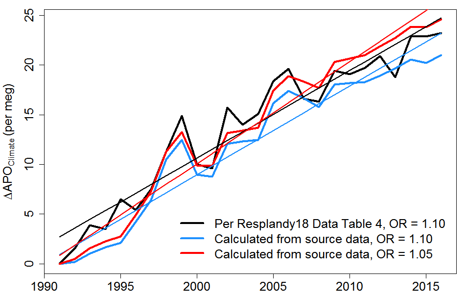
I have also not been able to replicate exactly the +0.15 change from changing the OR value from 1.10 to 1.05. Calculating the effect of the new OR assumption on ΔAPOClimate requires recalculating all the other ΔAPO time series, which in turn necessitates using their source data for O2 and CO2 concentrations and for fossil fuel emissions.[5] When I did so, the estimated ΔAPOClimate time series changed from that in Resplandy18’s Extended Data Table 4. Their ΔAPOClimate time series increases more slowly as time progresses, whereas my calculated time series increases somewhat more linearly. The change in the ΔAPOClimate time series is almost entirely due to my calculated ΔAPOObs time series differing from that in Resplandy18. It is unclear whether Resplandy18 made a (presumably uncorrected) error in their ΔAPOObs calculations or whether I did something contrary to what was specified in their Methods section.[6] My calculated ΔAPOObs time series is arguably more logical than Resplandy18’s, which more strongly indicates ocean heat uptake slowing (the OHC trend declining) over time, contrary to what in situ temperature measurements suggest.[7] Although the absolute OHC trend estimated by their ΔAPO method is very uncertain, their method should provide much less uncertain estimates of changes in OHC trend.
Although my calculated ΔAPOClimate values were lower in most years that those in Resplandy18, with a 1.10 OR value the mean OLS linear trend estimate was marginally higher than for Resplandy18’s ΔAPOClimate values: 0.89 rather than 0.88 per meg per year (Figure 4). When the OR value was changed to 1.05 ± 0.05, the OLS linear trend became 1.03 ± 0.69 per meg per year – close to the revised trend of 1.05 ± 0.62 per their correction, but still with higher uncertainty. The corresponding estimated trend in OHC is 1.18 ± 0.79 ⤬ 1022 J/yr, slightly lower and rather more uncertain than their revised estimate of 1.21 ± 0.72.
Figure 4. Mean estimate ΔAPOClimate time series as originally stated in Resplandy18 and as calculated by me from source data, both based on Resplandy18’s original oxidative ratio (OR) of 1.10, and as calculated by me based on their revised 1.05 OR value. Thin straight lines show the OLS linear fits to the corresponding time series.
My calculated ΔAPOClimate uncertainty estimate is 10% or so higher than their revised estimate. Ralph Keeling refers to their having originally incorrectly treated systematic errors in the O2 measurements, which they have presumably dealt with in their correction. However, I believe that Resplandy18 also seriously underestimated systematic errors in the ΔAPOFF (fossil fuel) time series, and that the correctly calculated uncertainty in its values is approximately double the values they gave.[8] When propagated to ΔAPOClimate time series values, this underestimation of ΔAPOFF systematic uncertainty would account for the 10% difference between their and my estimate of the OHC trend uncertainty range. I believe that they will need to revise their correction accordingly.
I turn now to the revision of the OR value used by Resplandy18. The only recent paper Ralph Keeling cited to justify reducing OR to 1.05 is Clay and Worral 2015,[9] which actually estimates a value of 1.06 ± 0.06. When using the Clay and Worral OR estimate, I calculate an ΔAPOClimate trend of 1.00 ± 0.69 per meg per year, and an OHC trend of 1.15 ± 0.80 ⤬ 1022 J/yr.
The case for changing the OR parameter may very well be valid, although while the correction provides a convenient opportunity for them to make this change I doubt that they would have done so otherwise. However, the sensitivity of the ΔAPOClimate trend to the OR value also helps illustrate how very uncertain the ΔAPOClimate trend actually is. They now conclude that:
The revised uncertainties preclude drawing any strong conclusions with respect to climate sensitivity or carbon budgets based on the APO method alone, but they still lend support for the implications of the recent upwards revisions in OHC relative to IPCC AR5 based on hydrographic and Argo measurements.
In fact, with the uncertainty range being so large, the ΔAPO based OHC trend estimates do not usefully discriminate between the AR5 estimates and more recent, generally higher, values. Moreover, even with the original, vastly underestimated, uncertainty range the conclusions that Resplandy18 drew with respect to (the lower bound of) climate sensitivity and carbon budgets were unwarranted, because estimated ocean heat uptake has little or no impact on either of these.
Conclusions
It is clear that the statistical method used in the original article resulted in a substantial overestimation of the trend in ΔAPOClimate, and hence of ocean heat uptake, and a vast underestimation of the uncertainty in those estimates. Using their uncertainty weights to obtain a linear WLS fit to the first differences of the ΔAPOClimate time series, as is appropriate given the nature of the errors in ΔAPOClimate, and correcting the omission of uncertainty in 1991, has major effects. The ΔAPOClimate trend estimate changes from 1.16 ± 0.15 to 0.89 ± 0.71 per meg per year. That is a 23% reduction in the central estimate and a near quintupling of estimated uncertainty. Correspondingly, the ΔOHC trend estimate changes from 1.33 ± 0.20 to 1.03 ± 0.82 ⤬ 1022 J/yr.
After their revision of the value used for the land oxidative ratio from 1.10 to 1.05 (± 0.05), the Resplandy18 authors estimate a ΔAPOClimate trend of 1.05 ± 0.62 per meg per year and a corresponding OHC trend of 1.21 ± 0.72 ⤬ 1022 J/yr, whereas I calculate estimates of 1.03 ± 0.69 per meg per year and 1.18 ± 0.79 ⤬ 1022 J/yr respectively. My estimates reduce further to 1.00 ± 0.69 per meg per year when the oxidative ratio of 1.06 (± 0.06) given in the recent paper cited by Keeling in support of their adoption of a revised OR value is used.
I believe that the remaining difference in our uncertainty ranges is likely due to the Resplandy18 correction failing to deal with a major underestimation of systematic uncertainty in ΔAPOFF. Moreover, I am unable to replicate the Resplandy18 ΔAPOObs time series, and hence also their ΔAPOClimate time series (although the ΔAPOClimate time series I compute has an almost identical linear trend to theirs); I think it possible that they may have miscalculated ΔAPOObs.
Nicholas Lewis 17 November 2018
Acknowledgements
I thank Ross McKitrick for very helpful statistical and other input to this article.
[1] I have taken the autocorrelation as ρ = 0.95, the value used in the reference Resplandy18 cite. Resplandy18 used an AR1 process to generate their random noise estimates on fossil fuel emissions; I did the same.
[2] WLS reduces to OLS if the error variances are equal.
[3] Application of a Goldfeld-Quandt test shows the error variances actually shrink over the sample, rather than growing, but not significantly. Application of a White’s test (even including the 1σ uncertainties as potential explanatory variables) also fails to detect heteroscedasticity.
[4] Application of a Breuch-Godfrey test fails to detect AR1 or higher order autocorrelation.
[5] The source Resplandy18 quote for fossil fuel emissions (Le Quéré, C. et al. Global carbon budget 2016. Earth Syst. Sci. Data 8, 605–649 (2016)) only gives values up to 2015. I took estimates for 2016 from the following year’s study, Global carbon budget 2017.
[6] It is not obvious where the difference could lie. The ΔAPOObs time series depends only on (δO2/N2) and CO2 data. Although it is highly sensitive to the source of CO2 concentration data, I took monthly (δO2/N2) and CO2 values measured at La Jolla, Alert and Cape Grim, the three stations specified in the Resplandy18 Methods section, weighting them respectively 0.25, 0.25 and 0.50 as per the reference they cited.
[7] The claim by scientist Paul Durack in the Washington Post that the Resplandy18 study confirms that the rate of ocean warming has been increasing is misleading, at best.
[8] This assertion is based on the oxidative ratios for each fossil fuel, and uncertainty ranges given for them and for CO2 emissions, in Resplandy18 Extended Data Table 3, which uncertainties are taken to be systematic rather than randomly varying each year. On that basis, it is simple to work out that the oxidative ratio uncertainties imply much higher uncertainty in ΔAPOFF than that stated in Resplandy18 Extended Data Table 4.
[9] https://www.sciencedirect.com/science/article/pii/S0341816214003129?via%3Dihub. The estimates they give for the two components of the global oxidative ratio indicate a slightly higher central estimate for it, of 1.067 ignoring rounding errors, so its unrounded value must lie above 1.06.


Leave A Comment