Originally a guest post November 23, 2018 at Climate Etc.
There have been further interesting developments in this story
Introduction
The Resplandy et al. (2018) ocean heat uptake study (henceforth Resplandy18) is based on measured changes in the O2/N2 ratio (δO2/N2) and CO2 atmospheric concentration. These are combined to produce an estimate (ΔAPOObs) of changes in atmospheric potential oxygen since 1991, from which they isolate a component (ΔAPOClimate) that can be used to estimate the change in ocean heat content. In three recent articles, here and here, and here, I set out why I thought the trend in ΔAPOClimate – and hence their ocean heat uptake estimate – was overstated, and its uncertainty greatly understated, essentially because of errors in their statistical methodology. These criticisms have been largely accepted by the authors of the study, although they have also made a change in an unconnected assumption that has the effect of offsetting much of the reduction in their ocean heat uptake estimate that correcting their statistical errors causes.
In the third article, I wrote that my calculated ΔAPOObs time series differed from that in Resplandy18, and said:
It is unclear whether Resplandy18 made a (presumably uncorrected) error in their ΔAPOObs calculations or whether I did something contrary to what was specified in their Methods section.
As I explained in an endnote, it was not obvious where the difference could lie. The ΔAPOObs time series depends only on (δO2/N2) and CO2 data. As it is highly sensitive to the source of CO2 concentration data, I took monthly (δO2/N2) and CO2 values measured at Alert, La Jolla and Cape Grim, the three stations specified in the Resplandy18 Methods section, weighting them respectively 0.25, 0.25 and 0.50 as per the reference they cited. These weights give equal weighting to the two hemispheres, only Cape Grim station being in the southern hemisphere.
Investigating the difference in ΔAPOClimate values
In order to investigate this issue, I turned to multiple regression. This was the approach that led me to suggest that GISS model simulations might have omitted land use forcing from their measure of total historical forcing, hence biasing the Marvel et al (2015)[1] estimates of its efficacy. While Gavin Schmidt responded in an article by asserting that “Lewis in subsequent comments has claimed without evidence that land use was not properly included in our historical runs”, my regression analysis provided good evidence of what I had suggested – which was subsequently bolstered by further evidence that I found – and proved to be correct. In the Resplandy18 case, the obvious thing to do was to regress the ΔAPOObs time series given in the paper on the three ΔAPOObs time series calculated, on the same basis as in Resplandy18,[2] for each individual station.
The results were surprising. They revealed that the influence, as measured by the relevant multiple regression slope coefficient, of the calculated ΔAPOObs data for the three stations differed greatly from the expected 0.25 for Alert and La Jolla and 0.50 for Cape Grim. The estimated coefficient for Alert was insignificant (not distinguishable from zero )! The estimated coefficients for La Jolla and Cape Grim were respectively 0.65 and 0.37, however these are only approximate as the regression fit was imperfect, with a residual standard error of ~ 0.8 per meg, leading to 1σ (1 standard deviation) uncertainty in these regression coefficients of 10–15% of their estimated value. This implied that the difference between my and Resplandy18’s ΔAPOObs time series couldn’t simply be due to a different set of weights having been used. Their data processing must differ from mine, with their weights not necessarily also differing from those indicated (although probably doing so), otherwise my regression would have obtained an excellent fit, albeit with different weights from {0.25, 0.25, 0.50}.
This seemed very strange, so I checked with Ralph Keeling whether they had used the {0.25, 0.25, 0.50} weights indicated in the paper’s Methods, being those cited in the paper that they cited in that connection.[3] He confirmed that was so. He also suggested that I double check the version of the data downloaded from the Scripps Institution website, as at point it had had a problem.
I re-downloaded the Scripps monthly O2 and CO2 data. The monthly data comes in four flavours. Two columns give the measured values before and after a seasonal adjustment to remove the quasi-regular seasonal cycle. There are a few missing data months, particularly for La Jolla where the prevalent wind direction in the winter sometimes results in there being no suitable sampling conditions during a month. The adjustment involves subtracting from the data a 4-harmonic function fit to the seasonal cycle. Two other columns contain a smoothed version of the data generated from a stiff cubic spline function, either with the 4-harmonic function added (thus containing a seasonal signal) or deseasonalised. The Resplandy18 Methods sections states:
Station annual means are based on bimonthly data fit to a four-harmonic seasonal cycle and a stiff long-term trend.
Although I was unsure why bimonthly data was referred to, I took this as meaning that the smoothed version of the monthly data was used; otherwise I would have expected the treatment of months with missing data to be mentioned. However, it was unclear to me whether the version of the smoothed data including or excluding the seasonal cycle had been used. I tried deriving annual mean (δO2/N2) and CO2 values from both versions of the smoothed monthly data – which gave essentially identical results – and various other alternatives, without being able to obtain a close regression fit.
As I couldn’t figure out what might be the cause, I went back to Ralph Keeling saying that although I found a strong dependence of the ΔAPOObs time series given in the paper on Cape Grim and (particularly) La Jolla data, I could not isolate any dependence on data from the Alert station, that there was a substantial amount of unexplained variance, and that it looked as if Alert station data might not have been processed as intended.
A surprising station weighting
Ralph Keeling quickly came back to me to say to he had just also figured out that Laure Resplandy had used different weights than he had thought. Shortly afterwards he confirmed that the actual weights used were {0.0105, 0.5617, 0.4278} for Alert, La Jolla and Cape Grim respectively. These weights not only differ very substantially from those indicated in the Methods section, but are physically inappropriate. Equal weighting the two hemispheres is important, and it makes no sense to put almost all the northern hemisphere weight on La Jolla, which unlike Alert station is close to human habitation and has considerably more months with missing data.
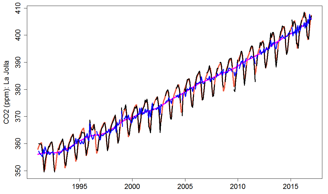
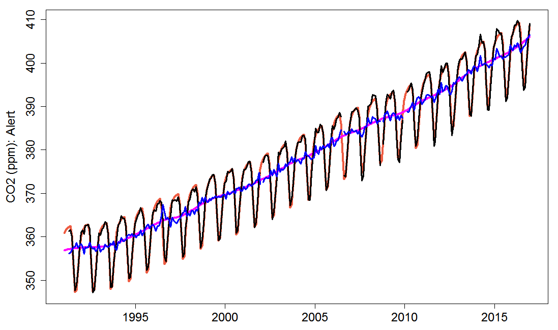
I imagine that Laure Resplandy misunderstood what the relevant statement in the Methods section meant and/or misunderstood the paper that it referenced, but I have no idea how she came up with the weightings that she used. Figures 1 and 2 show the four types of monthly CO2 concentration data at La Jolla and Alert stations respectively. The unsmoothed data shows substantially more fluctuation around the smoothed data at La Jolla than at Alert. At Cape Grim, in the southern hemisphere, there is very little such fluctuation.
Figure 1. Monthly CO2 concentration at La Jolla station. The black line shows raw monthly-mean measurements, the blue line shows them after the fitted seasonal cycle has been removed. The orange and magenta lines show the smoothed version with and without the inclusion of the fitted seasonal cycle.
Figure 2. As Figure 1 but for Alert station.
An unexpected derivation of ΔAPOClimate annual means.
Ralph Keeling helpfully provided me with the annual mean data that Laure Resplandy had used, explaining that he suspected I was working with data with messed up monthly values, and that it was possible the data posted on the web had not yet been fixed. He said that months with missing data get filled from the fit. This appears to be contrary to what the paper’s Methods section states, which implies that values from the fit (to a four-harmonic seasonal cycle and a stiff long-term trend) are used for all months, not just for months with missing data. Moreover, I’m not sure that mixing smoothed and unsmoothed data in this way is a good idea, particularly as data is preferentially missing in particular months.
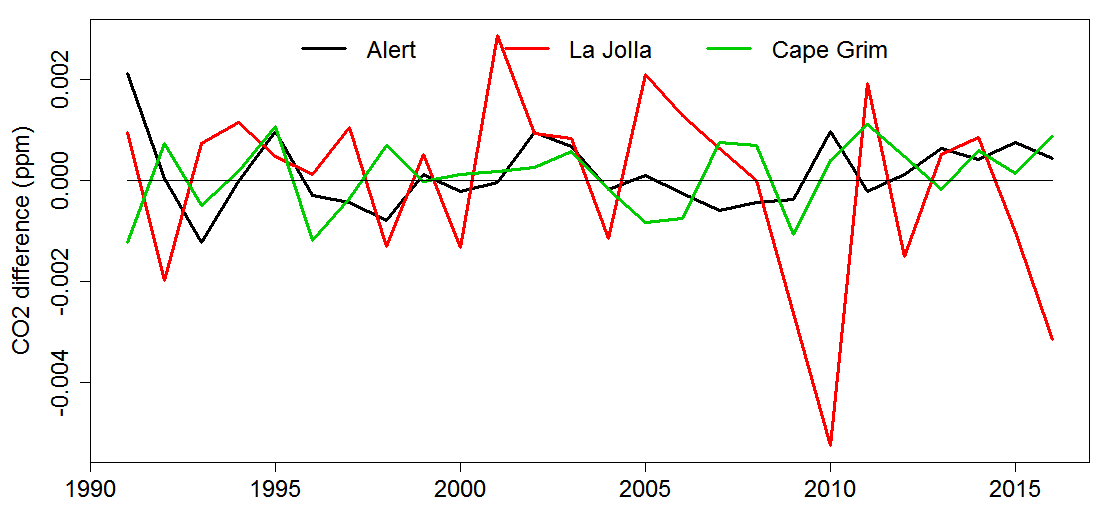
I found that I could almost exactly reproduce the annual O2 and CO2 time series Ralph Keeling sent from the monthly data I had downloaded, using the deseasonalised but unsmoothed version with missing months infilled with smoothed data from the version of the fit without the seasonal cycle. The differences (Figure 3) were only a few parts per billion for CO2, although somewhat less minute for La Jolla than the other stations. Examination of the mean values of this data for each month reveals that the seasonal cycle has not been completely removed, particularly for La Jolla.
Figure 3. Differences between the annual CO2 data provided by Keeling and that I calculate from downloaded data using the method he described, rather than that indicated in the Methods section.
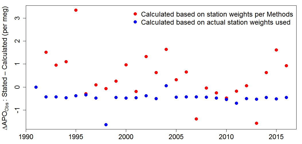
Strangely, despite now having, and being able to replicate, the annual O2 and CO2 data that Ralph Keeling said had been used, and knowing the actual weights used, I still could not very accurately reproduce the ΔAPOObs time series given in the paper; the RMS error is 0.55 per meg. Figure 4 shows the remaining differences (blue circles). A difference in the baseline 1991 value might account for the offset of approaching −0.5, and rounding errors for the remaining difference in most years, but there are larger differences in 1998, 2004 and 2011. The differences between the time series in Resplandy18 and that calculated using the station weights indicated in its Methods section are much larger (red circles). However, whichever basis of calculation is used the 1991–2016 trend of the resulting time series is almost the same, so there is only a minor effect on the resulting ΔAPOClimate trend and the ocean heat uptake estimate.
Figure 4. Differences between the ΔAPOObs annual values stated in Resplandy18 Extended Data Table 4 and those calculated using the CO2 data provided by Ralph Keeling, either giving the measuring stations the weights indicated in the Methods section or the actual weights used.
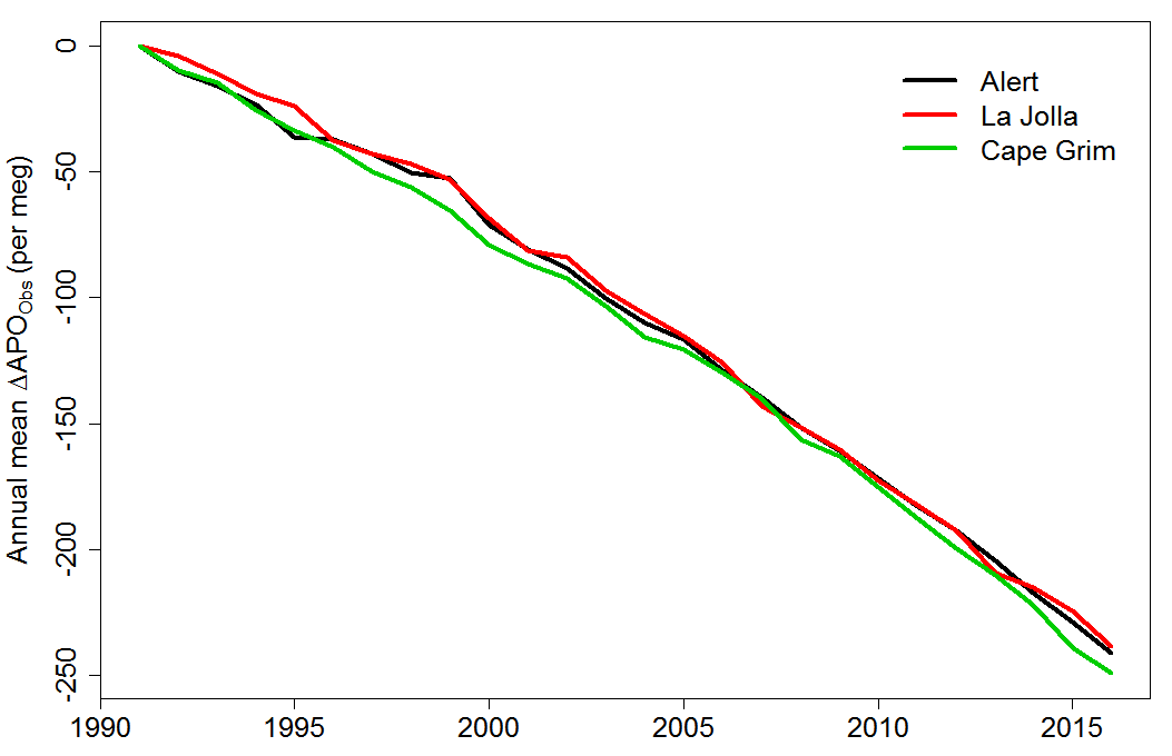
The development of ΔAPOObs for the three stations, calculated from the downloaded data on the basis actually used in Resplandy18, is shown in Figure 5. Trends calculated using the smoothed data, as stated in the paper’s Methods section, are almost identical. While the ΔAPOObs trend difference between the Alert and La Jolla stations looks small, it equates to a nearly 20% difference in the ΔAPOClimate trend and hence in the ocean heat uptake estimate.[4]
Figure 5. Annual mean ΔAPOObs time series for the three stations calculated from downloaded data using the method Keeling described.
As it happens, the effect of the very low weight, relative to that per the weightings indicated in the paper’s Methods section, given by Laure Resplandy to Alert (which has the weakest downwards trend) was largely cancelled out by the lower than indicated weight she gave to Cape Grim (which has the strongest downwards trend). Accordingly, the overall effect on the weighted-mean ΔAPOObs trend of the station weightings used differing from those indicated in the paper’s Methods section is minor.
Conclusions
Neither the station weighting nor the method used to derive annual means makes a material difference to the ΔAPOClimate trend and hence to the ocean heat uptake estimate. They nevertheless illustrate why publication of computer code is so important. In this case, the Methods section was commendably detailed, but in reality the derivation of annual mean O2 and CO2 data and the weighting given to data from the three stations used was different from that indicated in the Methods, radically so as regards the station weighting. It is possible, although hopefully not the case, that there are other differences between the stated methods and those actually used. With Resplandy18, I was lucky in that it was not too difficult to work out that there was a problem and in that Ralph Keeling has behaved very professionally, cooperating with my attempts to resolve the differences between the ΔAPOObs time series I calculated and those given in the paper. But a problem arising from the stated methods not actually being used can often only be revealed if code is made available. I have written to Nature making this point.
While the issues relating to the calculation of ΔAPOObs have now largely been clarified, there remain unresolved issues with the calculation of ΔAPOFF and the uncertainty in it. I shall be pursuing these.
Nicholas Lewis 23 November 2018
[1] Kate Marvel, Gavin A. Schmidt, Ron L. Miller and Larissa S. Nazarenko: Implications for climate sensitivity from the response to individual forcings. Nature Climate Change DOI: 10.1038/NCLIMATE2888. The simulations involved were CMIP5 Historical simulations by the GISS-E2-R model and associated diagnostics.
[2] As ΔAPOObs = δO2/N2 + (XCO2 − 350) ⤬ 1.1 / XO2 per meg, where XCO2 is CO2 concentration in ppm, XO2 = 0.2094, 1.1 is the value taken for the land oxidative ratio (OR) and the result is stated as the change from the 1991 ΔAPOObs value. All ΔAPO values in this article use an OR value of 1.1, as in the original Resplandy18 paper, not the revised 1.05 (± 0.05) OR value that Ralph Keeling has stated is used in their Corrigendum.
[3] Hamme, R. C. & Keeling, R. F. Ocean ventilation as a driver of interannual variability in atmospheric potential oxygen. Tellus B Chem. Phys. Meterol. 60, 706–717 (2008): Table 1 Global station weightings for 3 stations starting in 1991 (rightmost column)
[4] All stated trends are derived using ordinary least squares regression.
Leave A Comment