Originally a guest post on August 15, 2016 at Climate Etc.
Last week, a U.S. federal court upheld the approach that the government uses to calculate the social cost of carbon when it issues regulations [link]. The models appear to have seriously overestimated the social cost of carbon.
Introduction and Summary
Integrated assessment models (IAMs) combine simple models of the carbon cycle and of the response of the climate system to changes in atmospheric carbon dioxide (CO2) concentration with models of economic growth that incorporate the effects of imposing a carbon tax. They calculate the resulting social utility after estimated damages from climate change and costs of measures adopted – as a result of the carbon tax – to abate CO2 emissions. The optimum time-varying carbon tax computed by IAMs, being that which maximises the discounted value of utility out to a specified end date, is equal throughout the period to the social cost of carbon (SCC). Results from IAMs are used by governments when deciding what carbon taxes to impose and/or levels of emission reductions to target.[1]
This article primarily concerns DICE, one of three IAMs used by the US Government in their assessment of the SCC,[2] which was developed by William Nordhaus. He has written a book chapter that provides a good introduction to IAMs in general and to DICE in particular.[3] The DICE model spans 2010 to 2309 in 5-year time steps, with the carbon tax being varied from 2015 on. In this article I am just concerned with the workings of the DICE climate module and I do not question the rest of the model.
Although I consider the values of equilibrium climate sensitivity (ECS) used in the DICE model and of the resulting transient climate response (TCR) produced by its climate module to be higher than justified by best estimates based on observations of the climate system, I do not challenge those values here. However, I will show the DICE climate module to be mis-specified, in the sense that the time profile of its temperature response to forcing is inconsistent with understanding of the behaviour of the actual climate system, as reflected in and simulated by current generation (CMIP5) atmosphere-ocean general circulation models (AOGCMs).
It has been shown that the evolution of global-mean temperature in AOGCMs may be well represented by a simple physically-based 2-box model, as used in DICE, with suitable choices of ocean layer depths for each box. However, I show here that the climate module parameter values used in DICE correspond to physically unrealistic ocean characteristics. In the DICE 2-box model, the ocean surface layer that is taken to be continuously in equilibrium with the atmosphere is 550 m deep, compared to estimates in the range 50–150 m based on observations and on fitting 2-box models to AOGCM responses. The DICE 2-box model’s deep ocean layer is less than 200 m deep, a fraction of the value in any CMIP5 AOGCM, and is much more weakly coupled to the surface layer. Unsurprisingly, such parameter choices produce a temperature response time profile that differs substantially from those in AOGCMs and in 2-box models with typical parameter values. As a result, DICE significantly overestimates temperatures from the mid-21st century on, and hence overestimates the SCC and optimum carbon tax, compared with 2-box models having the same ECS and TCR but parameter values that produce an AOGCM-like temperature evolution.
My analysis shows that if the parameters of the DICE climate module are altered from their standard settings so as to be consistent with AOGCM behaviour and actual ocean characteristics, but leaving its ECS and TCR values unchanged, the SCC and optimum carbon tax follows a substantially lower trajectory (a quarter to a third lower, up to 2110), with greater CO2 emissions but a lower peak level of warming. The present value of utility is improved by up to $19 trillion, depending on which alternative parameter set is used. When using these parameter sets, a loss of utility of the order of $1 trillion results from imposition of the higher carbon tax that is optimum when using the DICE climate module standard settings instead of their own, lower, optimum carbon tax. The climate response profile in FUND[4] and in PAGE,[5] the other two IAMs used by the US government to assess the SCC, appear to be similarly inappropriate, suggesting that they also overestimate the SCC.
The climate module in the current version of DICE
I use the latest version of DICE, DICE-2013R (April 2014), the geophysical modules of which are stated to be largely consistent with the IPCC Fifth Assessment Working Group I report (AR5). It is stated to be in final form.[6] However, the Excel version available for download[7] does not incorporate a number of parameter revisions that were made in the primary, GAMS language, October 2013 version DICE2013Rv2 of the model, according to its manual.[8] Of particular relevance to its climate response are a reduction of the default ECS used, from 3.2°C to 2.9°C, and revisions in other climate module parameters. I have incorporated these changes, and parameter revisions in other parts of the DICE model that affect emissions and the SCC, in an updated Excel version that I refer to as DICE-2013Ra.[9] The manual states (page 18) that a change in a climate module parameter[10] was made to set the transient temperature sensitivity, as estimated by a regression analysis, at 1.70°C. It is confirmed elsewhere[11] that this sensitivity is intended to be the same measure as the TCR in AOGCMs, being the increase in global mean surface temperature (GMST) at the end of a seventy year period, starting from equilibrium, during which CO2 concentration rises at 1% p.a. compound, thereby doubling.
The DICE climate module represents a standard global 2-box climate model,[12] [13] in which the atmosphere is in continuous equilibrium with a surface mixed layer of the ocean that exchanges heat with the deep ocean at a rate proportional to the difference in temperature between them. This simple model is fully defined by specifying the ECS, the heat capacities CSO and CDO of the ocean surface and deep layers respectively, and the coefficient of proportionality FSD between the rate of interlayer exchange of heat and the interlayer temperature differential.[14] Alternatively, the value of FSD is uniquely determined if the TCR of the model is specified as well as its ECS.
Characteristics of 2-box climate models
The time varying change T(t) in GMST in the model in response to a step change in radiative forcings, such as one caused by a jump in atmospheric CO2 concentration, is given by the weighted sum of two exponential functions with time constants τ1 and τ2:
T(t) = k1 (1 – exp[–t/τ1] + k2 (1 – exp[–t/τ2])
The sensitivity factors k1 and k2 determine how the final, equilibrium GMST response (to which they sum) is divided between two component responses with differing time constants. A derivation of the mathematical relationships between the 2-box model physical parameters and the resulting exponential function time constants and sensitivity factors is given by Berntsen and Fuglestvedt (2008).[15] Generally, for given values of ECS and FSD, the heat capacity of the ocean surface mixed layer, CSO, which is proportional to its depth, strongly positively influences the value of τ1, whilst that of the deep ocean, CDO, strongly positively influences τ2. The relative values of k1 and k2 are strongly influenced by FSD. When formulating 2-box models, the surface layer that is in equilibrium with the atmosphere is typically taken to have a depth of 70–120 m, averaged over the ocean area, corresponding broadly to estimates of the mixed-layer depth.[16] Whilst the mean depth of the ocean is approaching 3,700 m, the effective depth for the purposes of a 2-box model may be smaller due to lesser heat exchange occurring below the bottom of the thermocline (the effective depth of which is of the order of 1,000 m). Consistent with these ocean characteristic depths, in 2-box models one expects τ1 to be a fairly short period – under ten years – and τ2 a long period – over a hundred years.
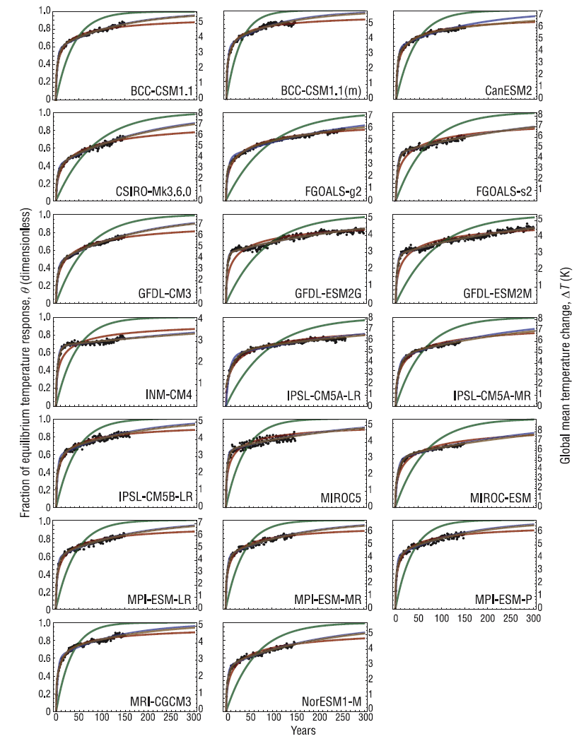
Although the 2-box climate model is very simple, the 2-exponential response it generates has been found able – with suitable parameter choices – to represent the GMST behaviour of AOGCMs remarkably well.[17] Figure 1 below, which reproduces Fig.2 of Caldeira and Myhrvold (2013),[18] shows how good 2-exponential fits (blue lines) are for CMIP5 models. Their investigation was based on the results of simulations in which atmospheric CO2 concentration was abruptly quadrupled, which provide a very clear picture of the characteristic time profile of model response to imposed forcing. The 2-exponential fits obtained from those simulations also provided excellent matches to the corresponding models’ GMST behaviour in 140 year ramp-forcing simulations where CO2 concentration was increased by 1% per annum.
Figure 1: GMST change in various CMIP5 models after an abrupt quadrupling of CO2 concentration at time zero (black dots), and as emulated by various simple models with best-fit parameter values. The blue lines represent fits to a 2-exponential response, as given by a 2-box model. In most cases they overlap with the 3-exponential fit brown lines. The olive green lines are for 1-exponential fits; the red lines for fits to a 1D diffusion model.
Consistent with physically-based expectations, Caldeira and Myhrvold found that the values of τ1 and τ2 giving the best fit varied in the ranges 2.4 – 7.4 and 109 – 463 years respectively, according to the CMIP5 model involved. The implied values of CSO and CDO correspond to ocean surface and deep layer depths ranging between respectively 64–150 m and 768–3313 m.[19] Another study involving CMIP5 AOGCMs, which contains more detail on 2-box models, reached similar conclusions; it also gave values for FSD, which ranged between 0.50 and 1.16 Wm-2K-1.[20] Likewise, Boucher and Reddy (2008) fitted a two-exponential model to the CMIP3 HadCM3 model and obtained time constants of 8.4 years for τ1 and 409.5 years for τ2, with sensitivity parameters equating to an ECS of 3.90°C and a TCR of 2.17°C.[21] Their fitted model was used in AR5.[22] Its implied values of CSO and CDO correspond to ocean surface and deep layer depths of respectively 142 m and 1600 m.[23] Berntsen and Fuglestvedt used somewhat different values for CSO and CDO, corresponding to a surface layer depth of 70 m and a deep layer depth of 3,000 m. The Boucher & Reddy and the Berntsen & Fuglestvedt ocean layer depth combinations span much of what is physically plausible (having regard to the depths of the ocean mixed layer, of the ocean below it and of the thermocline) and required to match CMIP5 model behaviour. Accordingly, I use the CSO and CDO value combinations from those two studies to define reference 2-box model variants, and compare their GMST responses with that of DICE-2013Ra. Whilst for each of these 2-box model variants the exponential time constants vary with the specified values of ECS and TCR, the ocean layer heat capacities and related depths remain unchanged.
Comparing the response of the DICE 2-box model with that of the two reference variants
To objectively compare the GMST responses of the different 2-box model parameterisations it is appropriate to specify the same ECS and TCR values for all of them. The differences in response will then depend only on the ocean surface and deep layer depths employed.
All parameters that affect TCR have the same values in DICE-2013Ra as in DICE-2013Rv2. Although Nordhaus states that the estimated TCR of DICE-2013Rv2 is 1.70°C, the value that I calculate for DICE-2013Ra, by applying a linear forcing ramp for 70 years from a preindustrial equilibrium position, is only 1.57°C.[24] The reason for the inaccuracy in the TCR setting in DICE-2013R is unknown; possibly it arises from the regression model used to estimate the model’s TCR being unsuitable.
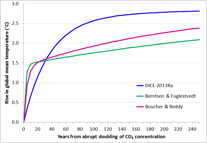
I accordingly set the values of FSD in the reference variants of 2-box models, with the Boucher & Reddy and the Berntsen & Fuglestvedt ocean surface and deep layer depths, so as to produce a TCR of 1.57°C when used in DICE-2013Ra, matching that with the model’s original settings, also retaining the same ECS value of 2.9°C. I then calculated, over 250 years, the GMST response of each 2-box model variant to an abrupt doubling of CO2 concentration; the results are shown in Figure 2. The shape of the response of DICE-2013a is notably different from that of the other two model variants. The shapes of the lines for the Boucher & Reddy and Berntsen & Fuglestvedt variants are similar to the blue 2-exponential curves, and to the actual AOGCM responses, in Figure 1, whilst the DICE-2013a line has a quite different shape – one closer to the green 1-exponential curves in Figure 1.[25] After 10 years, the CMIP5 AOGCM responses in Figure 1 have reached between 38% and 61% of their estimated ultimate, equilibrium, warming. After 100 years, they have reached between 60% and 86% of their equilibrium warming. The 10 year percentages for the Boucher & Reddy and Berntsen & Fuglestvedt models are respectively 44% and 51%; at 100 years they are 67% and 61%. These values lie within the ranges for the Figure 1 AOGCMs. However, the 10 and 100 year percentages for DICE-2013Ra, at 22% and 89% respectively, lie outside the AOGCM ranges.
Figure 2: GMST response of each 2-box model variant to an abrupt doubling of CO2 concentration
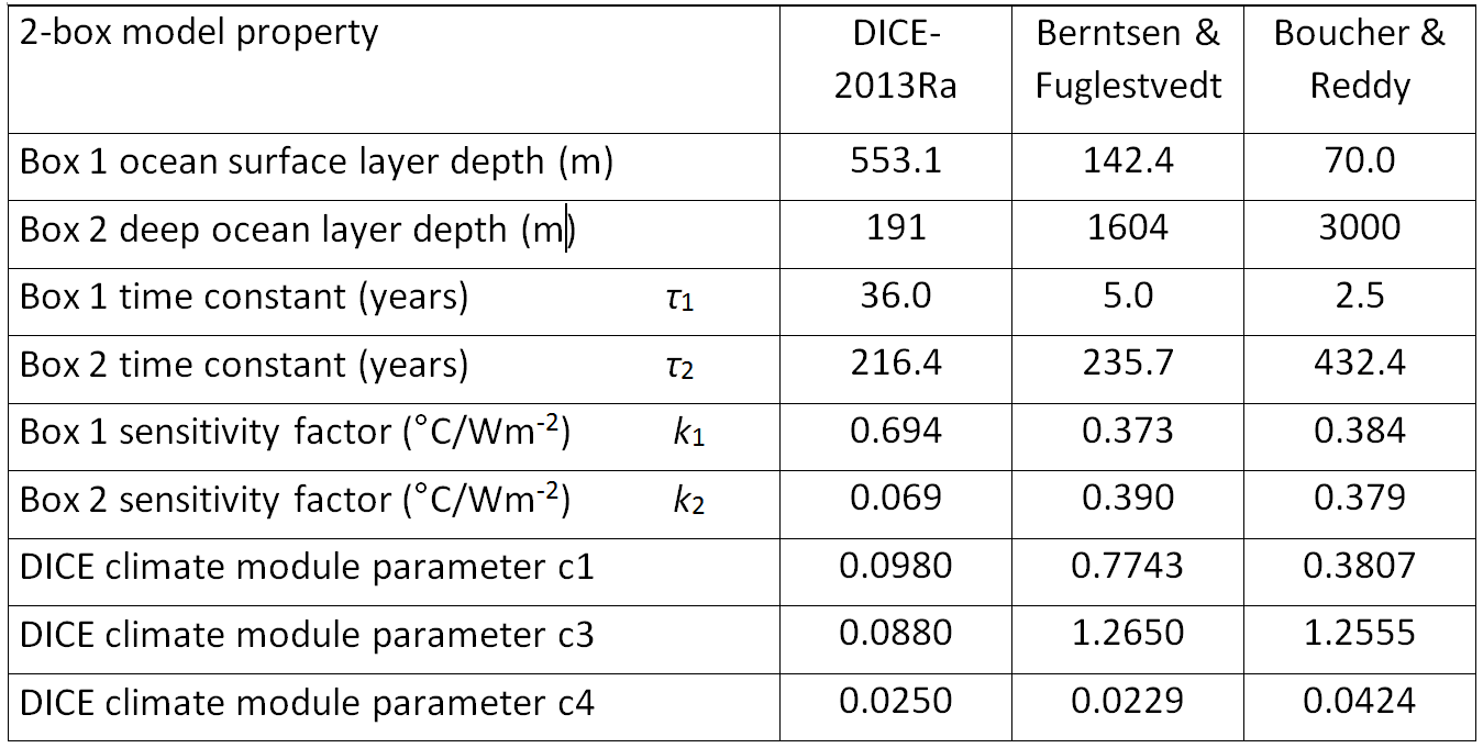
The reason for the abnormally shaped GMST response in DICE2013Ra is that its 2-box climate model embodies physically unrealistic ocean layer depths. Its implicit CSO value equates to a mean depth for the ocean surface layer of 553 m – four to eight times higher than for the two reference model variants, and far greater than the depth of the layer that is in near equilibrium with the atmosphere. The DICE-2013a CDO value equates to a mean depth for the deep ocean layer of 191 m – only a twelfth to a sixth of that in the other two model variants. DICE-2013Ra also has a much lower coefficient of heat exchange between the surface and deep ocean layers: its FSD value of 0.088 Wm-2K-1 is under 10% of that in the other two model variants (which have almost the same FSD values as each other).
As a result of the very weak surface to deep ocean coupling, the DICE-2013Ra second exponential term’s time constant is reasonable (216 years) despite the small depth of the deep ocean layer. However, its first exponential time constant, τ1, is extraordinarily high at 36 years, which is way outside the 2.4 – 7.4 year CMIP5 range found by Caldeira and Myhrvold. For the reference model variants, τ1 is 5 years for Boucher & Reddy and 2.5 years for Berntsen & Fuglestvedt. In DICE-2013Ra, the GMST response is dominated by that of the first exponential term; due to the weak inter-box coupling the longer time constant second term only contributes 9% of the total equilibrium warming.[26] This is far below the 33–61% range reported by Caldeira and Myhrvold for CMIP5 models, and compares with values of approximately 50% for both the Boucher & Reddy and Berntsen & Fuglestvedt based 2-box model variants.
Relevant details of all three 2-box model variants are given in Table 1.
Table 1: Properties of each 2-box model variant, all with ECS at 2.9°C and TCR at 1.57°C, the values corresponding to the default DICE-2013Ra parameters.[27]
The effect on the SCC and optimum carbon tax of the different 2-box climate models
The peculiar GMST response of the DICE-2013Ra 2-box climate model is much slower initially than that of the two much more physically-plausible alternative 2-box model variants, and than CMIP5 models, but its slope declines much more slowly. By 35 years after a forcing is applied, the DICE-2013Ra temperature response to an imposed forcing has overtaken that of the alternative 2-box model variants with identical ECS and TCR values, and by year 100 it is well above their responses.
The key question is what effect the varying shapes of these three climate response functions, all with identical values for both ECS and TCR, have on the SCC, on the CO2 emission pathways that follow from imposing an optimum carbon tax – one equal to the SCC – and on the present value of everyone’s utility. In order to be able to optimise the carbon tax using the standard Excel solver, which is unreliable for optimising more than a few parameters, I specify the carbon tax by a four parameter model.[28] I leave the savings rate values in the downloaded Excel model unchanged; the optimum savings rate is little affected by the variations in the optimum carbon tax.
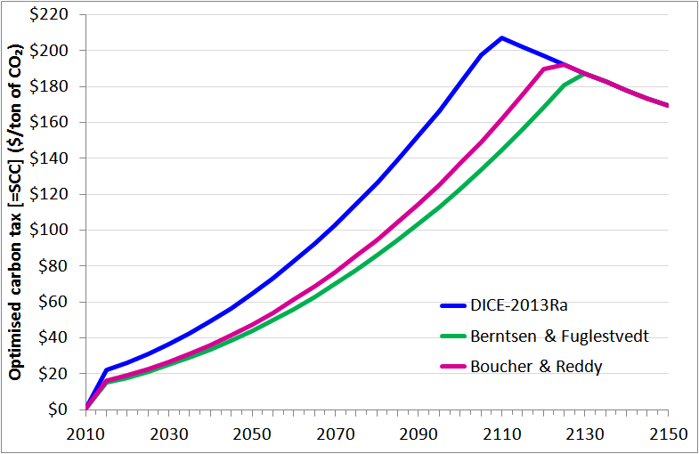
Figure 3 shows the resulting optimised carbon tax values with each 2-box climate model variant. Optimisation is applied from 2015 on; the initial 2010 carbon price is $1 in all cases. The peaks occur when the increasing SCC reaches the backstop price, an initially very high price that declines over time, at which any required amount of emission reduction is assumed to be possible.[29] Beyond 2150, in all cases the carbon price continues to decline with the backstop price.[30] Until 2110, the optimum carbon tax for the Berntsen & Fuglestvedt 2-box model variant is two-thirds, and that for the Boucher & Reddy variant is three-quarters, of that for the DICE2013Ra one.[31] These are substantial reductions.
Figure 3: DICE-2013Ra optimum carbon tax profile for each 2-box model variant
The effects of the different carbon tax levels on CO2 emissions, CO2 concentration and GMST
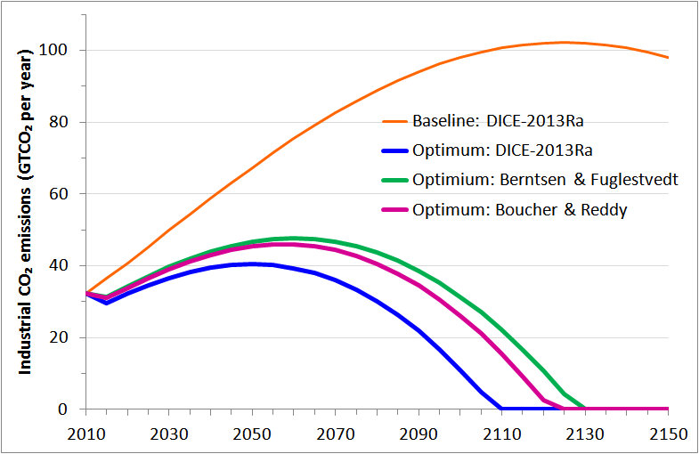
A lower carbon tax implies that optimum emissions are higher. Figure 4 shows the profile of CO2 emissions in each case that result from imposing the corresponding optimum carbon tax, and for comparison in the base case where the carbon tax increases only slowly from its 2010 level.[32] The cumulative 2010-2150 emissions in the three cases are 621, 790 and 858 GTCO2 – all far lower than the 2,222 GTCO2 in the base case. However, the emissions for the Berntsen & Fuglestvedt based 2-box model variant are 38% higher, and those for the Boucher & Reddy case 27% higher, than when based on the DICE2013Ra 2-box model.
Figure 4: DICE-2013Ra CO2 emissions with carbon tax optimised for each 2-box model variant
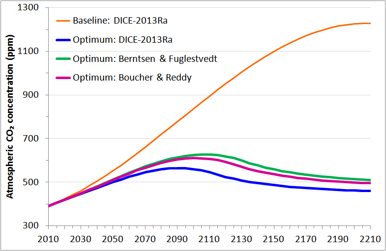
The corresponding atmospheric CO2 concentrations are shown in Figure 5, through to 2295. They peak about 60 ppm higher in the Berntsen & Fuglestvedt case than with the DICE-2013Ra 2-box climate model, reflecting the substantially higher cumulative CO2 emissions, but at only 51% of the baseline case peak level.
Figure 5: DICE-2013Ra CO2 concentration with carbon tax optimised for each 2-box model variant
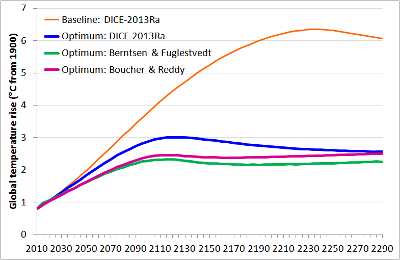
It might be thought that with the CO2 concentration being continuously higher with the Berntsen & Fuglestvedt and Boucher & Reddy based 2-box model variants than with DICE-2013Ra’s own 2-box climate model, the resulting increase in GMST would be greater in their cases. In fact, that is not so up to 2300. Indeed the peak GMST rise is noticeably higher with the native DICE-2013Ra climate model, at 3.0°C in 2120, at which time the rise is 2.5°C in the Boucher & Reddy case and 2.3°C in the Berntsen & Fuglestvedt case. Although in those two cases GMST ultimately rises further, in both cases it remains below 2.8°C for at least a thousand years. By comparison, in the baseline case the peak GMST increase is over 6°C.
Figure 6: DICE-2013Ra GMST change with the carbon tax optimised for each 2-box model variant
Discussion and conclusions
I have shown that the 2-box climate temperature response function used in DICE-2013R is unreasonable, as it is based on the ocean surface layer that is in equilibrium with the atmosphere being over 550 m deep, coupled very weakly to a deep ocean layer only 190 m thick, and has only 9% of the equilibrium response attributable to the exponential term with a centennial time constant. These values are neither physically realistic, having regard to actual ocean characteristics, nor compatible with the range of values implied by 2-box models that well-match the responses of CMIP5 AOGCMs. The abnormal characteristics of the DICE2013Ra 2-box model cause its estimated SCC and optimum carbon tax to be one third to one half too high over the first hundred projection years, depending on which of two more physically plausible alternative 2-box model variants considered, both having the same ECS and TCR values as DICE-2013Ra, is used. Thereafter the carbon tax rapidly converges on the same value, declining with time, in all cases.
Qualitatively similar comparative results are obtained if the DICE-2013Ra climate module parameter specified in the manual (c1) is adjusted to achieve a TCR of 1.70°C, the value that was apparently intended, its parameters also being adjusted to achieve that TCR for the other two 2-box climate model variants. The optimum carbon tax profile is higher, and the resulting CO2 emissions profile lower, in all three cases. The depth of the ocean surface layer in DICE-2013Ra is slightly lower, at 476 m, than with the default parameter values – still several times higher than is physically realistic or within the range of values required to match the behaviour of CMIP5 models. The proportion of the equilibrium response attributable to the exponential term with a centennial time constant in DICE-2013Ra is almost unaffected by the change in TCR; it remains unrealistically low at 9%.
It may be asked why the optimum carbon tax is higher, and hence the level of emissions lower, when the vast bulk of the GMST response comes from the box 1 exponential term, with a time constant of several decades, rather than being more evenly split between two exponential terms, with time constants of respectively well under a decade and over a century. The primary reason is that in the first case the increased forcing produced by emissions, which peaks around 2090 with the DICE-2013Ra carbon tax profile, causes a much greater increase in GMST in the second and third centuries than it does in the second case. Additionally, almost all of the substantial warming in-the-pipeline as at 2010, of 0.83°C,[33] emerges over the projection period in the first case, whereas in the second case a substantial fraction of it remains unrealised after 300 years.[34]
For a rational economist or policymaker, the relevant target might be expected to be the present value (PV) of total utility, discounted over the 300 year time horizon – exactly the target that the optimum carbon tax maximises. In the base case, DICE2013Ra calculates the PV of utility as 2,678.6 (all utilities are in trillions of year 2000 $). With the optimum carbon tax and its own climate model, the PV of utility increases to 2,707.0. If the Boucher & Reddy based 2-box model variant is used instead, the PV of utility rises further, to 2,722.8. If the Berntsen & Fuglestvedt based variant is used, the PV of utility becomes 2,726.0, or $19.0 trillion above the level using the DICE-2013Ra 2-box model. Of greater practical concern is the loss of utility if the higher carbon tax that is optimum when using the DICE climate module standard settings is imposed, when the actual climate response is in line with a more realistic 2-box model. For the Berntsen & Fuglestvedt based variant, this utility loss is $1.1 trillion; it is $0.7 trillion for the Boucher & Reddy based variant.[35] A loss of $1 trillion in the present value of utility equates to about a thirtieth of the total utility attributable to world consumption for the single year 2010.
The climate response profiles in FUND and in PAGE, the other two IAMs used by the US government to assess the SCC, also appear to be inappropriate. They both use one exponential term with the single time constant being of the order of 40 years, so no part of the temperature response has a centennial timescale (versus 9% in DICE-2013Ra). It therefore seems likely that they likewise significantly overestimate the optimum carbon tax at any given level of ECS and TCR, although detailed investigation would be required to confirm this.
It seems rather surprising that all three of the main IAMs have climate response functions with inappropriate, physically unrealistic, time profiles. In any event, it is worrying that governments and their scientific and economic advisers have used these IAMs and, despite considering what ECS and/or TCR values or probability distributions thereof to use, have apparently not checked whether the time profiles of the resulting climate responses were reasonable.
Nicholas Lewis
[1] See, e.g., https://www3.epa.gov/climatechange/EPAactivities/economics/scc.html.
[2] Technical Support Document: Technical Update of the Social Cost of Carbon for Regulatory Impact Analysis Under Executive Order 12866 Interagency Working Group on Social Cost of Carbon, United States Government
[3] Nordhaus, W. Integrated Economic and Climate Modelling. In Dixon, P.B., Jorgenson, D.W. (Eds.) Handbook of Computable General Equilibrium Modeling. Elsevier (2013) aida.wss.yale.edu/~nordhaus/homepage/documents/Nordhaus_IntegratedAssessmentModels_Handbook_2013.pdf
[4] Anthoff D and RSJ Tol. The Climate Framework for Uncertainty, Negotiation and Distribution (FUND), Technical Description, Version 3.9 (2014) www.fund-model.org/Fund-3-9-Scientific-Documentation.pdf
[5] Hope, C. The PAGE09 integrated assessment model: A technical description. Cambridge Judge Business School Working Papers 4/2011, University of Cambridge (2011) https://www.jbs.cam.ac.uk/fileadmin/user_upload/research/workingpapers/wp1104.pdf
[6] http://aida.wss.yale.edu/~nordhaus/homepage/
[7] DICE-2013 model, beta version of April 22, 2013, developed by William Nordhaus, Yale University. aida.wss.yale.edu/~nordhaus/homepage/documents/DICE_2013R_112513m.xlsm
[8] The new parameter values are given on page 96–97 of the Second edition( 31 October 2013) of the DICE-2013R manual, available at: aida.wss.yale.edu/~nordhaus/homepage/documents/DICE_Manual_103113r2.pdf . The reduction in the default ECS is discussed on page 18 of the manual.
[9] Climate module parameter c1 has been changed from 0.104 to (at the default ECS of 2.9°C) 0.098, and c3 from 0.155 to 0.088. I have also incorporated the following other changes per the DICE-2013Rv2 GAMS code in the manual: in Initial atmospheric temperature in 2010, from 0.83°C to 0.80°C; Initial carbon emissions from land use, from 1.53972 to 3.3 GTCO2/yr; in Initial atmospheric concentration of CO2 (used for 2010), from 384.50 to 389.86; in Initial output, from 66.95 to 63.69 2005 $ trillion; in Industrial CO2 emissions for 2010, from 8930 to 9168 MTC; in forcings of non- CO2 GHGs from −0.06 in 2000 and −0.62 in 2100 to 0.25 in 2010 and 0.75 in 2100 (Wm-2); and in the Damage coefficient on temperature squared, from 0.002131 to 0.00267. Minor other differences in the abatement module have been left untouched, as has the growth of population , which differs only marginally between the Excel and GAMS versions.
[10] Parameter c1, also termed ξ1 in the manual and there wrongly referred to as the diffusion parameter and overstated there by a factor of ten.
[11] Nordhaus, W. Integrated Economic and Climate Modelling, op. cit., p.1088.
[12] Gregory JM, Vertical heat transports in the ocean and their effect on time-dependent climate change. Clim Dyn (2000) 16:501±515.
[13] Held, I. M. et al, Probing the fast and slow components of global warming by returning abruptly to preindustrial forcing. J. Climate, 23 (2010), 2418–2427.
[14] The heat capacity of the atmosphere and land is small relative to that of the ocean mixed layer, and is subsumed within the value used for it.
[15] Berntsen, T and J Fuglestvedt. Global temperature responses to current emissions from the transport sectors. PNAS 105 (2008), 19154–19159. See the Supplementary Information.
[16] The annual maximum depth of the ocean surface mixed layer is relevant here.
[17] It might be thought that a 1D model in which heat is transferred diffusively between a surface mixed layer and thermocline/ deep ocean, with slow upwelling linked to sinking cold water in polar regions often also being included, would be more appropriate. However, as much of the heat is believed to be transported between ocean layers by advection of water along sloping isopycnal surfaces (Gregory 2000, op. cit.) the simpler 2-box model treatment appears to be satisfactory.
[18] Caldeira K and N P Myhrvold. Projections of the pace of warming following an abrupt increase in atmospheric carbon dioxide concentration. Environ. Res. Lett. 8 (2013) 034039 (10pp)
[19] Ricke K and Caldeira D. Maximum warming occurs about one decade after a carbon dioxide emission Environ Res Lett 9 (2014) 124002 doi:10.1088/1748-9326/9/12/124002
[20] Geoffrey et al (2013) carried out a similar exercise with a different, overlapping set of CMIP5 models and found good fits, with the values of τ1 and τ2 giving the best fit varied in the ranges 1.6 – 5.5 and 126 – 698 years respectively. Geoffroy O et al. Transient Climate Response in a Two-Layer Energy-Balance Model. Part I: Analytical Solution and Parameter Calibration Using CMIP5 AOGCM Experiments J. Clim. 26 (2012) 1841–57
[21] Based on the HadCM3 forcing for a doubling of CO2 concentration of 3.68 Wm-2.
[22] The Global Temperature change Potentials given in Table 8.A.1 of AR5.
[23] For the ocean only, based on the ocean covering 71% of the Earth’s surface and a seawater volumetric heat capacity of 4.1 M J K-1 m-3.
[24] Moreover, the theoretical TCR I calculate using the two-box model parameters is only 1.51°C. The difference appears to be due to use of a 5-year time step and to applying forcing increments at the start of each period. When a 1-year time step is used, the TCR calculated from applying a 70-year forcing ramp is only 0.01°C above the theoretical value.
[25] If the surface ocean depth in the Boucher & Reddy based variant is swapped with that in the Berntsen & Fuglestvedt based one and the FSD values altered to maintain their TCRs, the shapes of the resulting response curves are almost bounded between those for the two versions with unswapped surface ocean depths over the entire 250-year period.
[26] The warming in the second term of the two exponential representation of a 2-box model is not the same as that of the deep ocean layer in the underlying physical model, which ultimately warms as much as the surface.
[27] In DICE-2013R, the forcing from a doubling of atmospheric CO2 concentration is 3.8 Wm-2, so the sum of the sensitivity factors for each model variant is 2.9/3.8 = 0.763
[28] The carbon tax model specifies an initial value, initial growth rate, and a rate of change of growth rate that increases by the same specified amount each year. Fixed reductions are applied in the final three periods, matching those in the downloaded Excel model (the reasons for which are unknown); doing so has a negligible effect on the present value of utility. When all parameter values are as in the downloaded model, optimising the four parameter fit produces an almost identical carbon tax profile to that in the downloaded model, which were derived by optimising each period’s carbon tax independently, and the present value of utility is unchanged to seven significant figures.
[29] Per the DICE manual, the backstop technology can replace all fossil fuels; it could be one that removes carbon from the atmosphere or an all-purpose environmentally benign zero-carbon energy technology. The downward trend in its price is based on assumed technological progress.
[30] Up to 2290, from when on the fixed reductions referred to in note 28 are applied.
[31] More precisely, 68% for Berntsen & Fuglestvedt and 73–76% for Boucher & Reddy.
[32] Land use change emissions, which in DICE20113R are assumed to decline on a fixed basis, are not included. In the base case the $1 initial carbon tax increases by 10.4% in each pentad until 2015, from when the backstop CO2 price is applied.
[33]The currently unrealised, “in-the-pipeline”, warming at the end of 2010 equals ECS of 2.9°C x Forcing in 2010 of 2.14 Wm-2 / Forcing for a doubling of CO2 of 3.8 Wm-2, minus Atmospheric temperature rise in 2010 above preindustrial of 0.8°C.
[34] 0.80°C of the 0.83°C unrealised warming as at 2010 emerges by the end of the projections when the DICE-2013Ra climate module parameters are used, but only 0.45°C or 0.60°C when parameters based respectively on the Berntsen & Fuglestvedt or Boucher & Reddy models are used.
[35] In the contrary cases, where the actual climate response is as per the DICE-2013Ra 2-box model but a lower carbon tax that is optimum for one of the two variants is imposed, the utility losses are a little (10-20%) larger. However, it is most unlikely that the DICE-2013Ra response could be realistic.
Leave A Comment