Originally a guest post on Jul 8, 2017 – 5:49 AM at Climate Audit
A new paper in Science Advances by Cristian Proistosescu and Peter Huybers “Slow climate mode reconciles historical and model-based estimates of climate sensitivity” (hereafter PH17) claims that accounting for the decline in feedback strength over time that occurs in most CMIP5 coupled global climate models (GCMs), brings observationally-based climate sensitivity estimates from historical records into line with model-derived estimates. It is not the first paper to attempt to do so, but it makes a rather bold claim and, partly because Science Advances seeks press coverage for its articles, has been attracting considerable attention.
Some of the methodology the paper uses may look complicated, with its references to eigenmode decomposition and full Bayesian inference. However, the underlying point it makes is simple. The paper addresses equilibrium climate sensitivity (ECS)[1] of GCMs as estimated from information corresponding to that available during the industrial period. PH17 terms such an estimate ICS; it is usually called effective climate sensitivity. Specifically, PH17 estimates ICS for GCMs by emulating their global surface temperature (GST) and top-of-atmosphere radiative flux imbalance (TOA flux)[2] responses under a 1750–2011 radiative forcing history matching the IPCC AR5 best estimates.
In a nutshell, PH17 claims that for the current generation (CMIP5) GCMs, the median ICS estimate is only 2.5°C, well short of their 3.4°C median ECS and centred on the range of observationally-based climate sensitivity estimates, which they take as 1.6–3.0°C. My analysis shows that their methodology and conclusion is incorrect for several reasons, as I shall explain. My analysis of their data shows that the median ICS estimate for GCMs is 3.0°C, compared with a median for sound observationally-based climate sensitivity estimates in the 1.6–2.0°C range. To justify my conclusion, I need first to explain how ECS and ICS are estimated in GCMs, and what PH17 did.
For most GCMs, ICS is smaller than ECS, where ECS is estimated from ‘abrupt4xCO2’ simulation data,[3] on the basis that their behaviour in the later part of the simulation will continue until equilibrium. That is because, when CO2 concentration – and hence forcing, denoted by F – is increased abruptly, most GCMs display a decreasing-over-time response slope of TOA flux (denoted by H in the paper, but normally by N) to changes in GST (denoted by T). That is, the GCM climate feedback parameter λ decreases with time after forcing is applied.[4] Over any finite time period, ICS will fall short of ECS in the GCM simulation. Most but not all CMIP5 coupled GCMs behave like this, for reasons that are not completely understood. However, there is to date relatively little evidence that the real climate system does so.
Figure 1, an annotated reproduction of Fig. 1 of PH17, illustrates the point. The red dots show annual mean T (x-coordinate) and H (y-coordinate) values during the 150-year long abrupt4xCO2 simulation by the NorESM1-M GCM.[5] The curved red line shows a parameterised ‘eigenmode decomposition’ fit to the annual data. The ECS estimate for NorESM1-M based thereon is 3.2°C, the x-axis intercept of the red line. The estimated forcing in the GCM for a doubling of CO2 concentration (F2×) is 4.0 Wm−2, the y-axis intercept of the red line. The ICS estimate used, per the paper’s methods section, is represented by the x-axis intercept of the straight blue line, being ~2.3°C. That line starts from the estimated F2× value and crosses the red line at a point corresponding approximately to the same ratio of TOA flux to F2× as currently exists in the real climate system. If λ were constant, then the red dots would all fall on a straight line with slope −λ and ICS would equal ECS; if ECS (and ICS) were 2.3°C the red dots would all fall on the blue line, and if ECS were 3.2°C they would all fall on the dashed black line. The standard method of estimating ECS for a GCM from its abrupt4xCO2 simulation data, as used in IPCC AR5, has been to regress H on T over all 150 years of the simulation and take the x-axis intercept. For NorESM1-M, this gives an ECS estimate of 2.8°C, below the 3.2°C estimate based on the eigenmode decomposition fit. Regressing over years 21–150, a more recent and arguably more appropriate approach, also gives an ECS estimate of 3.2°C.
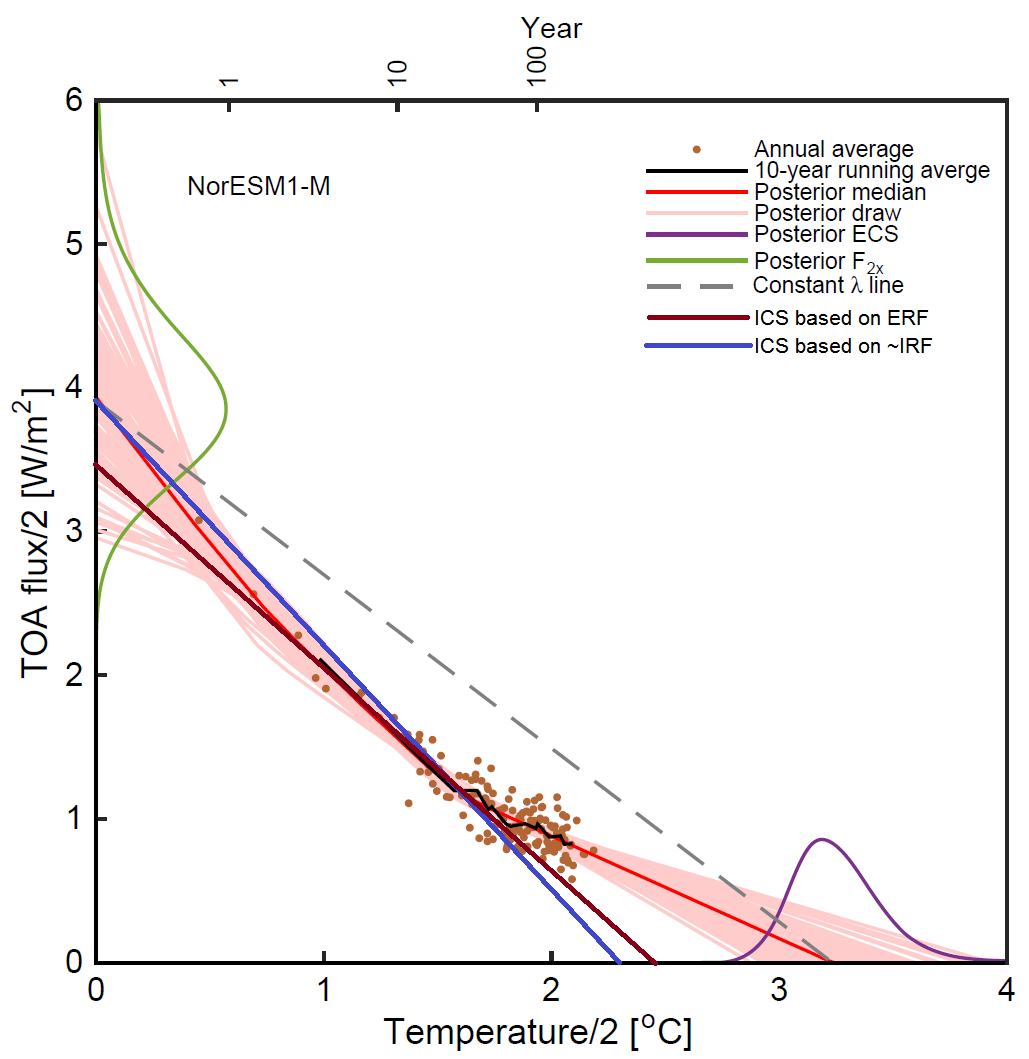
Fig. 1. Reproduction of Fig. 1 of PH17, with added brown and blue lines illustrating ICS estimates
Observationally-based climate sensitivity estimates derived from instrumental data are determined as ICS, since the climate system is currently in disequilibrium, with a positive TOA flux imbalance.
The most robust observational estimates of climate sensitivity based on instrumental data use an “energy budget” approach, described in IPCC AR5. That is they estimate the ratio of the change in GST to that in total forcing net of TOA flux imbalance, and scale the resulting estimate by F2× to convert it to ICS, as an approximation to ECS. To minimise the impact of measurement errors and internal climate system variability, these changes are usually taken between decadal or longer base and final intervals early and late in the instrumental period. The intervals chosen should be well matched in terms of volcanic activity (which has different effects from other forcing agents) and multidecadal Atlantic variability. Both Otto et al 2013 (estimate based on 2000s data) and Lewis and Curry 2015 satisfied these requirements. Otto et al used a GCM-derived forcing time series adjusted to match the overall change per IPCC AR5; Lewis & Curry used forcing time series from AR5 itself. Their observationally-based ICS median estimates were respectively 2.0°C and 1.6°C.
PH17’s statement: “A recent review of observationally based estimates of ICS shows a median of 2°C and an 80% range of 1.6° to 3°C” is based on a sample of 8 studies that included outdated and/or unsound ones. A number of other sound observationally-based ICS estimates not included in the sample used by PH17 fall within the 1.6–2.0°C range spanned by the Otto et al and Lewis & Curry estimates (Ring et al 2012 1.8°C; Aldrin et al 2012 1.76°C; Lewis 2013 1.64°C; Skeie et al 2014 1.67°C; Lewis 2016 1.67°C). I consider 1.6–2.0°C more representative than 1.6–3.0°C of the range of median ICS observationally based estimates from high quality recent studies.
PH17 uses an energy budget method to estimate ICS. If the energy-budget method is applied, based on the evolution of forcing over the historical period, to a GCM in which λ decreases with time, as in Figure 1, the resulting ICS estimate will obviously be lower than the GCM’s estimated ECS. However, contrary to what PH17 claims, if ICS is estimated using sound methods then the underestimation relative to ECS is typically modest, and the median CMIP5 model ICS estimate is still well above ICS for the real climate system as estimated by the best quality instrumental studies.
At this point I need to explain the eigenmode decomposition fitting method used in PH17. Eigenmode decomposition is just a fancy name for the standard method of representing the T and H responses of a GCM at time t to the imposition of a step doubling of CO2 concentration, producing forcing F2×, as the sums of several exponentially-relaxing terms with different time constants (τi) and amplitudes. (αi for T; βi for H). Mathematically, illustrating a case with three-eigenmodes, as in FH17:
T(t) = α1 [1 − exp(−t/τ1)] + α2 [1 − exp(−t/τ2)] + α3 [1 − exp(−t/τ3)]
F2×− H(t) = β1 [1 − exp(−t/τ1)] + β2 [1 − exp(−t/τ2)] + β3 [1 − exp(−t/τ3)]
Rearranging the second equation, and substituting λi αi for βi, gives:
H(t) = λ1 α1 exp(−t/τ1) + λ2 α2 exp(−t/τ2) + λ3 α3 exp(−t/τ3)
where ECS = α1+ α2+ α3 and F2×= β1 + β2 + β3 = λ1 α1 + λ2 α2 + λ3 α3.
Since the T and H response to forcing appears to be very linear in GCMs, these formula can be used to derive T and H responses to any forcing time series, by convolving the forcing time series with the time varying responses per these formulae and scaling down by the F2× value given by the final formula.
The ECS estimate is the sum of the amplitudes for the T terms, and the F2× estimate is the sum of the amplitudes for the H terms.[6] The time constants are specified to be the same for T and H. If the amplitudes for T and H are required to be in the same ratio for each time constant, this corresponds to a multi-box ocean global physical model of the climate system with constant λ. If they are not required to have the same ratio and only two time constants are allowed, it corresponds to a 2-box model in which λ may vary with time.[7] PH17 fits a three time-constant model with no restrictions on the ratios of the T and H amplitudes. Such a model can well fit the abrupt4xCO2 T and H responses of all CMIP5 GCMs.[8]
The (subjective) Bayesian methods discussed in PH17 are just used to optimise the fitted amplitude and time constant values for each GCM. Although they use informative priors, I doubt that these introduce much bias, since the signal-to-noise ratio of abrupt4xCO2 simulation data is quite high.[9] I suspect that the estimation method may lead to overstatement of uncertainty in GCM ICS values, but in this article I focus on median estimates so that is not relevant.
ICS calculation
In PH17, ICS was inferred by applying total historical forcing F (per AR5 median estimate time series) over 1750–2011 to the estimated eigenmode fits for each GCM, thus deriving emulated time series of its H and T values. This was done 5,000 times for each GCM, sampling from the derived posterior probability distribution for the eigenmode fit parameter values. The 2.5°C estimate for GCM-derived ICS is the median across the 24 GCMs of all the sample ICS estimates – 120,000 in all.[10] This approach seems very reasonable in principle, but the devil is in its detailed application.
PH17 states that ICS is obtained as F2×/λ(t), where λ(t) = (F − H)/T, with F, H and T being departures in 2011 from preindustrial conditions. Each of F, H and T is taken to have zero value in preindustrial conditions; total 1750 forcing was zero in the AR5 time series and the initial simulated values of H and T are zero.
PH17 also states that as values of F2× associated with each posterior draw could vary from the 3.7 Wm−2 assumed in the AR5 estimate of historical forcing, they multiplied F by F2×/3.7 for each draw before obtaining the values of H and T. While doing so is logical, it actually has no effect on the derived value of λ, since the multiplier scales equally both the numerator and denominator of the fraction representing λ. What is, however, critical to correct estimation for ICS for a GCM is that the F2× value into which the estimated λ is divided is, as implied by PH17, the estimated F2× for that particular GCM (which will vary between samples), and not some other value, such as the 3.7 Wm−2 used in AR5. Per PH17 Table S1 the median estimated GCM F2× values range from 2.9 to 5.8 Wm−2.
Error in ICS calculation
Cristian Proistosescu has very helpfully provided me with a copy of his data and Matlab code, so I have been able to check how the PH17 ICS values were actually calculated. Unfortunately, it turns out that the calculation in PH17 is wrong. Although for each GCM and each set of its sample eigenmode parameters, PH17’s code scales the AR5 forcing time series by the F2× value corresponding to its sampled eigenmode parameters (and thus also scales the related simulated H and T time series), it then divides the resulting λ estimate into 3.7 Wm−2 rather than into the F2× value applicable to that sample. Essentially, what PH17 did was to correctly estimate the slope of the blue line but, instead of estimating ICS directly from its x-axis intercept, they shifted the blue line down so that its y-axis intercept was 3.7 Wm–2.. In the case shown in Figure 1, doing so reduces the ICS estimate from 2.3°C to 2.1°C.
I have rerun the PH17 code with the ICS calculation corrected, applying the F2× value applicable to each sample to compute the ICS estimate for that sample. The resulting overall median ICS estimate increases from 2.5°C to 2.8°C. The 2.5°C value found by PH17 is quite clearly incorrect.
Volcanic Forcing
The corrected median ICS estimate for GCMs of 2.8°C, based on changes over the entire 1750-2011 period, is still a little below the value I would have expected from previous work of mine using rather similar methods. The reason for this is the incorrect treatment of volcanic forcing in PH17. The points involved are quite subtle.
The problem is that PH17 did not adjust the AR5 forcing time series to make average volcanic forcing zero. If one does not do so, that implies preindustrial (natural only) forcing was on average negative relative to that in 1750 (when all forcings, including volcanic forcing, are set at zero in the AR5 time series), meaning that in 1750 the climate system (which is assumed to be in equilibrium with pre-1750 average forcing) would not be in equilibrium with 1750 forcing (which is higher by the negative of average pre-1750 natural forcing. That would invalidate the PH17 derivation of (F − H)/T and hence of ICS. Although average pre-1750 natural forcing values are not given in AR5, it is reasonable to estimate them from the average over 1750–2011. That average is negligible for solar forcing, but material for volcanic forcing, at −0.40 Wm–2.
The need to account for preindustrial volcanic forcing when computing subsequent warming is known,[11] although it appears to have been overlooked by many GCM modellers. A simple solution is to adjust the AR5 forcing time series so that it has a zero mean over 1750-2011. This is essentially the same approach as was used when the RCP scenario forcing time series were produced. The volcanic forcing in 1750 then becomes +0.4 Wm–2, reflecting unusually low volcanism in that year.
When I adjusted the AR5 forcing time series by subtracting the average volcanic forcing over 1750–2011, the ICS median estimate over 1750-2011 rose to 2.92°C.
The appropriateness of the volcanic forcing adjustment can be seen by comparing median ICS estimates based on the 1750–2011 period with those based on differences between averages over base and final intervals matching those used in observationally-based studies. PH17 gives median ICS values using intervals of 1860-1879 and 2000-2009 (stated to be following Gregory et al 2002, but actually as in Otto et al 2013), and also for 1859-1883 and 1995-2011 (stated to be following Otto et al 2013, but actually matching Lewis & Curry 2015 except that it used 1882 not 1883). It also gives a median ICS value based on change between 1955 and 2011 (stated to be following Roe and Armour 2011, but actually matching the analysis period used by Masters 2014). All of these estimates were 2.6°C; they varied by under 0.01°C and on average they were nearly 0.07°C higher the median ICS estimate based on the 1750–2011 change. That reflects the fact that much of the mismatch between 1750 forcing and climate state that occurs when unadjusted volcanic forcing is used has washed out of the system by the 1850s, although the slowest time constant (several century) mode will have only partially adjusted. When volcanic forcing is adjusted, the shortfall of the median 1750-2011 ICS estimate over those based on the later intervals becomes much smaller. The average of those three ICS estimates is 2.94°C, only 0.02°C higher than that based on 1750-2011.
IRF versus ERF
There is a third reason why the PH17 estimate of ICS for GCMs is too low.
When CO2 concentration is abruptly doubled, it initially produces what is termed instantaneous radiative forcing (IRF). However, for estimating the response of the climate system it is best to use effective radiative forcing (ERF), which is forcing after the atmosphere has adjusted and surface adjustments that do not involve any change in GST have taken place; see IPCC AR5 Box 8.1. Such adjustments take up to a year, perhaps more, to complete. The IPCC AR5 forcing series are for ERF, and adopt an F2× value of 3.71 W m–2. ERF for CO2 is believed to be some way below IRF.
However, in PH17, F2× is estimated by projecting back to time zero using, primarily, mean values for the first and second years of the abrupt 4xCO2 simulations. Since during year one the atmosphere and surface are adjusting (independently of GST change) to the quadrupling in CO2 concentration, doing so produces a F2× value that is in excess of ERF. Thus, PH17 derives a median GCM F2× of ~4 Wm–2 (the median values for λ and Contribution to inferred equilibrium warming given in Table 1, imply, in conjunction with the median GCM ECS given in Table S1, an F2× value of 4.0 Wm–2).
It is difficult to estimate ERF F2× for CO2 very accurately from abrupt 4xCO2 simulation data. A reasonable method is to use regression over years 1 to 20 of the abrupt 4xCO2 simulation,[12] which is consistent with the recommendation in Hansen et al (2005)[13] of regressing over the first 10 to 30 years. The ensemble median F2× obtained by doing so is the best part of 10% lower than per PH17, although the ratio for individual GCM medians varies between 0.72 and 1.20. To obtain an apples-to-apples comparison, the F2× values implicit in the fitted model eigenvalue parameters must be for ERF, as for observationally-based estimates, not for something between ERF and IRF. The brown line in Figure 1 illustrates the issue. The intersection of the blue and brown lines corresponds to where we are now, in terms of how long the climate system has had on average to adjust to forcing increments during the historical period (scaled to a doubling of CO2 concentration). The brown line corresponds to estimating ICS using the same data relating to the current climate system state as for the blue line, but with the F2× estimate reduced from PH17’s 4.0 W m–2 to 3.6 Wm–2. The result is to increase the ICS estimate by approaching 0.2°C – the difference between the x-intercept of the brown and the blue lines. I cannot accurately estimate the depressing effect on ICS estimation of using F2× estimates that exceed those corresponding to ERF, as doing so would require refitting the statistical model and obtaining fresh sets of 5,000 sample eigenmode fits for each GCM.[14] However, based on my previous work I estimate the effect to be ~ 0.1°C. When this is added to the 2.94°C median ICS estimate, after correcting the two problems previously dealt with, for time periods used in instrumental-observation studies the median GCM based ICS estimate would slightly exceed 3.0°C.
Other issues
There are a few other points relevant to appraisal of PH17.
The PH17 calculations of T for CMIP5 GCMs using AR5 forcing time series reveal that, for the median fitted eigenmode parameters, simulated warming between 1860–79 and 2000–09 was 1.10°C.[15] That exceeds recorded warming (using a globally-complete GST dataset)[16] of 0.84°C by almost a third, supporting the conclusion that the median GCM is substantially too sensitive.
It is also worth noting that, although of considerable interest in relation to understanding climate system behaviour, any difference between ICS and ECS is of relatively little importance when estimating warming over the next few centuries on scenarios involving continuing growth of emissions and CO2 concentrations, as the slow mode will contribute only a small part of the total warming.
Finally, there are a number of fairly obvious errors and inconsistencies in PH17.[17] It is difficult for the person who writes a paper to spot such errors, but the fact that no reviewer did so suggests that its peer review was not very rigorous.
Conclusions
When correctly calculated, median ICS estimate for CMIP5 GCMs, based on the evolution of forcing over the historical period, is 3.0°C, not 2.5°C as claimed in PH17. Although 3.0°C is below the median ECS estimate for the GCMs of 3.4°C, it is well above a median estimate in the 1.6–2.0°C range for good quality observationally-based climate sensitivity estimates. PH17’s headline claim that it reconciles historical and model-based estimates of climate sensitivity is wrong.
Nic Lewis
PS Cristian Proistosescu has seen a draft of my above post. He does not, at least at present, accept my arguments in relation to what is the correct F2× value to use when deriving the ICS estimate from the computed λ value relating to a set of sample eigenmode parameters.
Update
Cristian Proistosescu has explained his reasons for thinking that it was appropriate to use an F2× value of 3.7 Wm–2 to calculate ICS for all eigenmode decomposition samples across all GCMs, rather than for each sample using its own F2× value, as follows:
“The amount of expected warming is a function of two components: the radiative feedbacks, and the radiative forcing.
The mechanism invoked to explain the discrepancy between historical and model estimates is a change in the net radiative feedbacks. Model net feedback was computed as (F − H)/T, as in the observations, after rescaling relative historical forcing to be commensurate with model F2× (needlessly in hindsight, as the net feedback only cares about the relative history of forcing, up to a multiplicative constant). Indeed, observations can constrain T and H, whereas the forcing history is diagnosed from a combination of models and observations. Thus, comparison of the net feedback between historical and model-derived estimates provides for a cleaner comparison between observations and models.
To report sensitivity as amount of warming, ICS studies use an AR5 F2x range that is quoted from the CMIP5 subset of models ran with Fixed SSTs (AR5 TS & 9.7.1). The same AR5 F2× value was used, since it would not be accurate to compare “observational” ICS that used an older and more restrictive model-derived F2×, and our study using an updated model derived F2×.”
There are several reasons why I disagree with this justification:
- Whatever the merits of comparing net feedback (λ) rather than estimated ICS between models and observations, PH17 claimed it compared ICS estimates, not λ estimates.
- In any event, the PH17 methodology doesn’t enable an unbiased comparison of λ values between models and observations. That is because, as I explained, observational estimates of (F − H)/T use estimated ERF values for F, including for the dominant CO2 forcing, whereas the PH17 eigenmode decomposition fitting method results in an F2× value somewhere between ERF and IRF – quite possibly closer to IRF, which exceeds ERF. If lower, ERF basis, F2× values were used when deriving net feedback in the GCMs, their estimated λ values would be lower (compare the slopes of the blue and brown lines in Figure 1) A fair comparison between GCMs and observations in terms of λ requires that their λ estimates both use an F2× estimate of the same nature, not ERF for observations and an IRF/ERF hybrid for models.
- The claim that observational ICS estimates used an older and more restrictive model-derived F2× is misleading. The AR5 F2× ERF value of 3.7 Wm–2 was derived from fixed SST simulations by ten CMIP5 GCMs. All ten of those models are included in the set of GCMs used in PH17. The median and mean of the F2× values estimated by PH17 for those ten models are both 4.0 Wm–2, exactly the same as for the full PH17 set of GCMs. So the subset is representative in this regard. But the median and mean Fixed SST estimates of F2× ERF for those ten models are both 3.7 Wm–2, 7.5% lower. There is no reason to think that the PF17 F2× estimates better reflect F2× for the real climate system than the 3.7 Wm–2 F2× ERF estimate given in AR5. Indeed, quite the opposite, since the PH17 methodology is not an appropriate one for estimating F2× on an ERF basis.
- All PH17 can hope to fairly estimate is what ICS estimated for GCMs would be for a time profile of radiative forcing that matches, in relative shape, the estimated historical forcing history, and to compare that with observational ICS estimates. That is, in my view, what a competent reader of PH17 would think the study does. It is implicit in consistent estimation of ICS for a GCM that if the forcing history is of a fixed forcing that has been applied for a period long enough for the GCM to reach equilibrium, the ICS estimate will equal the estimated ECS for the GCM. I have tested this using the PH17 sampled eigenmode decomposition fits, applying a fixed forcing for 5,000 years. When using the original PH17 code, for each the resulting ICS median estimate does not agree to its estimated ECS; on average the equilibrium ICS estimates are somewhat lower than the ECS values. Using my modified code that applies each sample’s F2× value to calculate ICS, for each GCMs the equilibrium ICS median estimate is in line with its estimated ECS.
- Finally, the most important point. The authors argue that it would not be accurate to compare observational ICS that used an older and more restrictive model-derived F2×, and their study’s ICS estimates for GCMs using an updated model derived F2×, which is on average higher than the older F2× used by observational studies. Let’s suppose that their median model derived F2× value of 4.0 Wm–2 did actually represent a valid, more up to date estimate of F2× ERF for the real climate system. They implies that substituting it for the AR5 F2× value of 3.7 Wm–2 would increase observational ICS estimates, narrowing the gap with ICS estimates for GCMs. In fact, doing so would if anything lead to lower observational ICS estimates, increasing the gap with ICS estimates for GCMs.How so? ICS is estimated as F2×/λ = F2× * T / (F − H), with F2× and F both using estimated ERF values. Now, F is dominated by CO2 ERF, and throughout recent decades (and throughout most if not all of the instrumental period) estimated CO2 ERF has exceeded (F − H). In the AR5 forcing time series, the CO2 ERF value for each year is 3.7 * log2(estimated CO2 concentration for the year/1750 CO2 concentration) Wm–2). While there is considerable uncertainty in F2×, the logarithmic change in CO2 concentration over the industrial period is accurately known; AR5 (Section 8.3.2.1) estimates its relative uncertainty to be an order of magnitude lower than that in F2× ERF. So, if the higher PH17 estimate of F2× = 4.0 Wm–2 had been used for AR5, the AR5 CO2 forcing time series would have used a multiplier of 4.0 rather than 3.7 to convert the CO2 concentration time series into forcing values. So, when deriving using F2× * T / (F − H) observational estimates of ICS that are consistent with AR5 F2× and forcing time series estimates but substituting the PH17 F2× value of 4.0 Wm–2, the (F − H) denominator would increase in at least the same proportion as the F2× multiplier increases. Accordingly, observational ICS estimates based on a revised F2× ERF estimate of 4.0 Wm–2 would be the same or lower than those based on the original AR5 F2× estimate of 3.7 Wm–2.
[1] ECS is defined as the increase in global surface temperature (GST) resulting from a doubling of atmospheric CO2 concentration once the ocean has fully equilibrated.
[2] The TOA radiative flux imbalance is measured downwards and is equal to the rate of planetary heat uptake.
[3] The abrupt4xCO2 simulations involve abruptly quadrupling CO2 concentration from an equilibrated preindustrial climate state; most such CMIP5 simulations were run for 150 years, but a few for up to 300 years. The use of abrupt4xCO2 simulation data to estimate the ECS of GCMs, most often by regression of TOA flux against GST change, is standard. Most GCMs have not been run to equilibrium with doubled CO2 concentration. Even where they have, any change in their energy leakage over time or with climate state would bias the resulting ECS value.
[4] The authors define λ as −ΔH(t)/ΔT(t), corresponding to the negative of the slope for the overall changes in H and T at time t after a forcing is imposed, rather than as −dH/dT|t, the negative of the instantaneous slope at time t.
[5] Values are changes from those in the equilibrated control simulation from which the abrupt4xCO2 simulation was branched, adjusted for drift and halved to restate for doubled CO2 concentration, making the assumption that for CO2 forcing is exactly proportional to log(concentration).
[6] PH17 scale the T amplitudes to sum to one, and do the same for the H amplitudes, but that is just for convenience.
[7] With λ varying in a manner corresponding to heat uptake by the deep ocean (represented by the second box, with the longer time constant) having non-unit efficacy – a different effect from a forcing of the same absolute magnitude. See Geoffroy et al. (2013, DOI: 10.1175/JCLI-D-12-00196.1) for a detailed explanation of this model.
[8] Less than perfectly for the Chinese FGOALS-g2 model; at least some of the CMIP5 simulations of which are known to be faulty.
[9] PH17 did test the sensitivity of eigenmode parameter estimates to changes in prior, and found them to be insensitive.
[10] The total sample size is slightly lower, since for eight of the GCMs the simulation method fails in a number of cases, due to use of an approximation that breaks down for samples with a very small fitted short time constant.
[11] Gregory et al 2013 doi:10.1002/grl.50339; Meinshausen et al 2011 DOI 10.1007/s10584-011-0156-z Appendix 2
[12] As in Andrews et al (2015, DOI: 10.1175/JCLI-D-14-00545.1)
[13] Efficacy of climate forcings, doi:10.1029/2005JD005776
[14] Probably requiring setting λ1 = λ2;it is impossible to estimate a separate λ1 if one seeks to estimate ERF, as the relevant time constant, τ1, is too short – typically less than a year.
[15] With volcanic forcing adjusted to zero mean over 1750-2011
[16] Cowtan and Way v2 kriged HadCRUT4v5: http://www-users.york.ac.uk/%7Ekdc3/papers/coverage2013/series.html
[17] Aside for the multiple errors in referenced studies relating to the various time intervals used for alternative ICS estimates, other errors and inconsistencies are as follows. The median GCM ECS is stated as 3.5°C in the text, but Table S1 shows it to be as 3.4°C (which calculation I have checked). Likewise the median time constant τ1 is given as 0.8 years in Table 1 but as 0.7 years in Table S1. And the statement that the F2× estimates for GCMs have a 90% credible interval range of 2.9 to 5.3 Wm–2 appears to be wrong; Table S1 shows a 90% range of 2.9–5.9 Wm–2, which appears to be correct.
Leave A Comment