A pdf version of this article is available here
An important new paper by Thorsten Mauritsen, Associate Professor at Stockholm University[i] and myself has just been accepted for publication (Lewis and Mauritsen 2020)[ii]. Its abstract reads:
Recently it has been suggested that natural variability in sea surface temperature (SST) patterns over the historical period causes a low bias in estimates of climate sensitivity based on instrumental records, in addition to that suggested by time-variation of the climate feedback parameter in atmospheric general circulation models (GCMs) coupled to dynamic oceans. This excess, unforced, historical “pattern effect” (the effect of evolving surface temperature patterns on climate feedback strength) has been found in simulations performed using GCMs driven by AMIPII SST and sea ice changes (amipPiForcing). Here we show in both amipPiForcing experiments with one GCM and through using Green’s functions derived from another GCM, that whether such an unforced historical pattern effect is found depends on the underlying SST dataset used. When replacing the usual AMIPII SSTs with those from the HadISST1 dataset in amipPiForcing experiments, with sea ice changes unaltered, the first GCM indicates pattern effects that are indistinguishable from the forced pattern effect of the corresponding coupled GCM. Diagnosis of pattern effects using Green’s functions derived from the second GCM supports this result for five out of six non-AMIPII SST reconstruction datasets. Moreover, internal variability in coupled GCMs is rarely sufficient to account for an unforced historical pattern effect of even one-quarter the strength previously reported. The presented evidence indicates that, if unforced pattern effects have been as small over the historical record as our findings suggest, they are unlikely to significantly bias climate sensitivity estimates that are based on long-term instrumental observations and account for forced pattern effects obtained from GCMs.
In this article I explain in more detail what Lewis and Mauritsen (2020) is all about and what its main findings and conclusions are. For a full picture, please read the paper, which is open-access; it is available in a reformatted version here.
Introduction
The back-story is concerns have been expressed that accounting for changing temperature patterns increases historical period energy budget based estimates of climate sensitivity.[iii] [iv] [v] This idea is now being used in assessments of climate sensitivity to increase significantly estimates based on historical period warming (e.g., Sherwood et al. 2020[vi]).
As I explained in a detailed 2018 article,[vii] the key paper making and quantifying this effect (Andrews et al 2018) was based on simulations driven by an observationally-based estimate of the evolution of SST and sea-ice over the historical period (amipPiForcing experiments, over 1871–2010), that showed, in six models, their climate feedback strength (λ, here λamip) on average to be substantially greater, and hence their effective climate sensitivity (EffCS[viii], here EffCSamip), substantially lower, than when responding to long-term CO2 forcing.
Only a relatively small part of the differences reported in Andrews et al. (2018) can be attributed to effective climate sensitivity to CO2 forcing increasing over time in most atmosphere-ocean global climate models (AOGCMs). Based on typical CMIP5 AOGCM behaviour, that factor, which is allowed for in some historical period energy budget based estimates, such as Lewis and Curry (2018)[ix], would only account for approximately 5% out of the 40% shortfall in effective climate sensitivity that Andrews et al. found,[x] with a further 7% due to their use of mismatching CO2 forcing values.7 This implies that the bulk of the average difference they found was instead attributable to unforced (internal) climate variability having affected SST patterns – a (positive) unforced historical pattern effect. Although I put forward arguments, both in Lewis and Curry 2018 and in my 2018 article, against claims of such an effect having occurred, such claims have become widely accepted by climate scientists.
There are other possible explanations for the differences reported in Andrews et al. (2018). One is that the AOGCMs’ simulated long-term SST and sea-ice patterns, and the resulting radiative responses, are unrealistic. Another is that the GCM radiative responses in amipPiForcing experiments are unrealistic. In this article I shall put those questions aside. A further possibility is that the forced response of the climate system to the historical mixture of forcings differs significantly from that to pure CO2 with the same time-profile of evolving effective radiative forcing. LC18 put forward evidence against that being the case. Moreover, I produced evidence in a subsequent article that, in the two models for which radiative response in standard CMIP5 climate model historical experiment was accurately known, there was no evidence that the response to the mix of anthropogenic forcings differed from that to pure CO2 forcing.[xi]
I wrote in my 2018 article that to justify the a existence of a dampening unforced historical pattern effect one would need – even assuming long-term SST and sea-ice patterns, and the radiative response to them, simulated by AOGCMs to be realistic – to establish:
- that correctly-calculated EffCSamip estimates are adequately robust to choice of historical SST and sea-ice observational dataset;
. - that the differences between climate feedback strength over the historical period in amipPiForcing simulations (λamip) and when AOGCMs generate their own SST and sea-ice patterns in response to radiative forcing (λhist) could feasibly be due to natural internal climate system variability.
It is standard to use the AMIPII SST and sea-ice dataset[xii] to drive GCMs in amipPiForcing experiments. The AMIPII sea-ice dataset is based closely on HadISST1 data throughout the historical period, with only minor modifications. However, the AMIPII SST dataset is only based on HadISST1 data until late 1981, after which it is based on OIv2 SST data[xiii]. The OIv2 post-1980 SST dataset is based largely on the same in situ and satellite data as HadISST1, but with different bias corrections and a different interpolation method for reconstructing SSTs in areas lacking in situ observations.
Andrews et al. (2108) showed, in their Supporting Information, that EffCSamip estimates are not robust to choice of historical sea-ice observational dataset. They found that climate feedback in amipPiForcing simulations by two UK Meteorological Office GCMs was much weaker – λamip was smaller, and hence EffCSamip was higher[xiv] – when the HadISST2 rather than the AMIPII sea-ice dataset was used, in conjunction with HadISST2 SST data. The difference was mainly due to the change in sea-ice data rather than in SST data, and was large enough to reverse the sign of the unforced historical pattern effect, making it negative.[xv] While sea-ice variation is thus an important contributor to differences in climate feedback, we do not explore sensitivity to sea-ice dataset in Lewis and Mauritsen (2020), caveating our results in that respect. Instead we use consistent sea-ice data, enabling isolation of the influence of SST dataset on historical climate feedback.
Thorsten and I show in our paper that λamip estimates are far from robust to choice of historical SST dataset, and that when the widely used HadISST1 dataset is used in place of the AMIPII SST dataset – with unchanged AMIPII sea-ice data – λamip and λhist are indistinguishable: no unforced historical pattern effect is found with the models we used. We also investigated the unforced historical pattern effect using five other SST datasets, finding a significant estimated effect only in one case.[xvi]
Although the Lewis and Mauritsen (2020) findings are based on simulations by only two GCMs, directly for ECHAM6.3 and indirectly (via “Green’s functions”) for CAM5.3,[xvii] they are consistent with historical warming in the Indo-Pacific warm pool, relative to that over the ice-free ocean as a whole, being much higher in the AMIPII than in the HadISST1 SST dataset.[xviii]
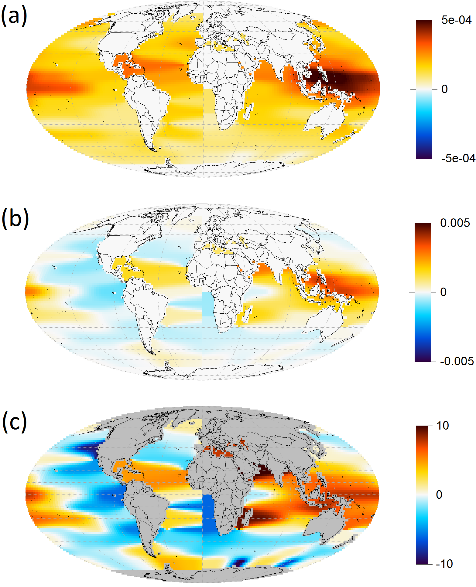
There is evidence, at least in CMIP5 models, that climate feedback strength is strongly positively related to relative warming in the Indo-Pacific warm pool.[xix] On physical grounds, warming in tropical ascent regions, of which the most important is the Indo-Pacific warm pool, relative to elsewhere is expected to produce a strong increase in outgoing radiation at the top of atmosphere.[xx] This effect, as estimated using the CAM5.3 Green’s functions, is illustrated in Figure 1 of our paper, reproduced below.
Figure 1. CAM5.3 Green’s functions: panels (a) and (b) show the change in respectively global mean Ts (K) and in global mean R (Wm−2) per 1K increase in local grid-cell SST, while panel (c) shows the global climate feedback parameter λ (Wm−2K−1) for a change in local grid-cell SST (the ratio of the values plotted in panel (b) to those plotted in panel (a)).
Our results
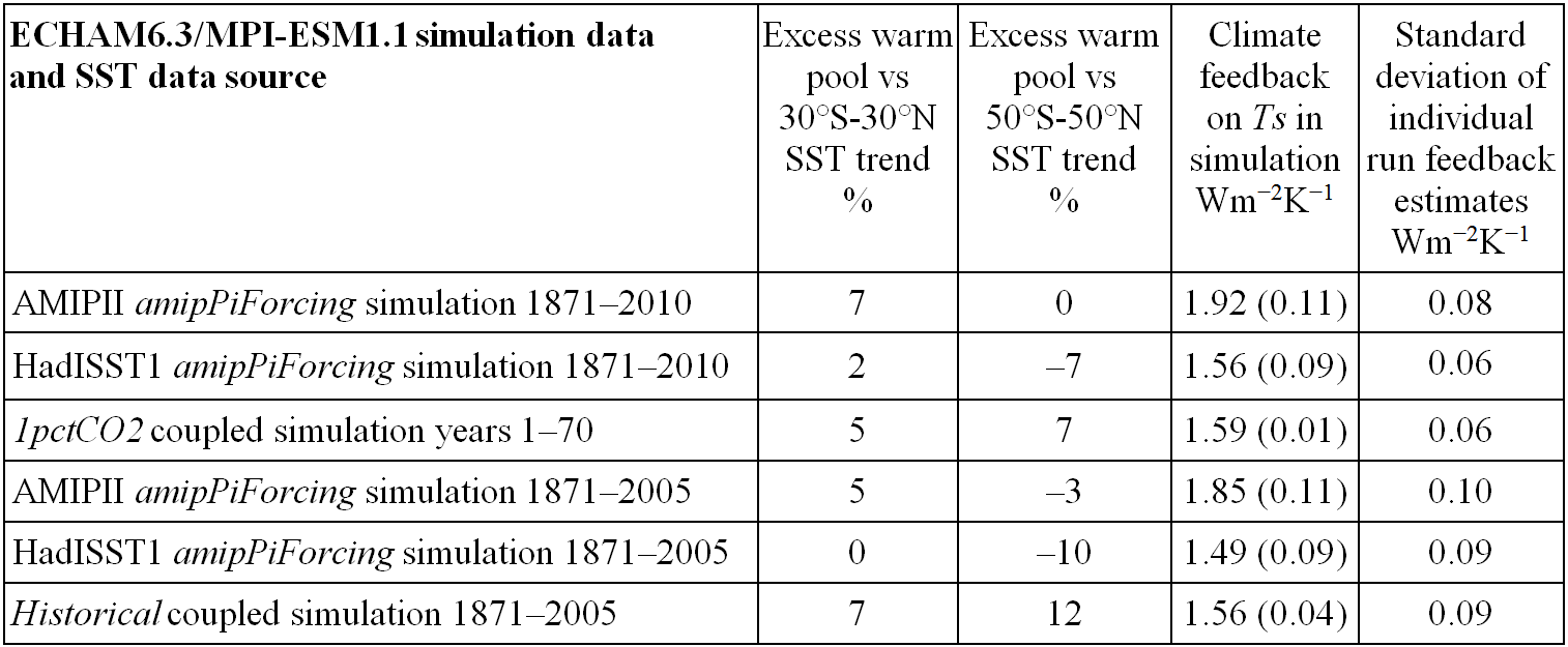
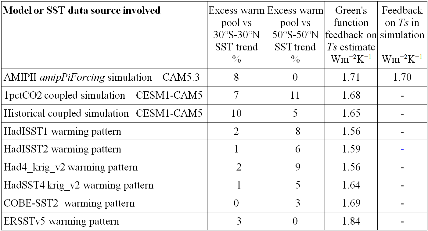
The Lewis and Mauritsen (2020) main results are set out in its Tables 1 and 2, reproduced below:
Table 1. Excess Indo-Pacific warm pool SST trends and climate feedback, in ECHAM6.3 amipPiForcing simulations and in MPI-ESM1.1 coupled 1pctCO2 and historical simulations. All values are based on ensemble mean Ts and R data (save for AMIPII and HadISST1 SST trends and standard deviations of individual run feedback estimates). Feedback estimates are from OLS regression, of pentadal mean data for amipPiForcing simulations. Values in brackets are standard errors of the OLS regression feedback estimates, which reflect underlying deviations from a linear relationship as well as internal variability.
.
Table 2. Excess Indo-Pacific warm pool SST trends and Green’s function derived estimates of climate feedback in CAM5.3 AMIPII-based amipPiForcing simulations, in CESM1-CAM5 coupled 1pctCO2 and historical/RCP8.5 simulations, and for warming in six observational SST datasets, along with feedback estimated from the actual CAM5.3 AMIPII-based amipPiForcing simulation data. Feedback estimates are from OLS regression of pentadal mean R and Ts values derived from the evolving SST warming patterns in the relevant simulation or observationally-based dataset. Data over 1871-2010, the amipPiForcing experiment period, is used, with data from the historical experiment extended using RCP8.5 experiment data, save in the 1pctCO2 simulation case where years 1–70 data is used.
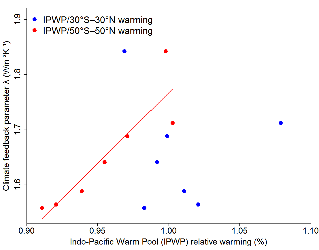
It has been found in CMIP5 AOGCMs that on average approximately 60% of the change in feedback parameter over time during abrupt4×CO2 simulations comes from the tropics (30°N–30°S),[xxi] due in particular to the west tropical Pacific warming significantly less than the east tropical Pacific, with the tropical pattern becoming more El Niño like as simulations progress. However, the Green’s function feedback estimates for the seven observationally-based SST datasets are strongly correlated with warm pool SST trends relative to those over the tropics and mid-latitudes (r=0.90), but not relative to those over the tropics alone (r=−0.10) (Figure 2).
Figure 2: a reproduction of Figure 4 of Lewis and Mauritsen (2020). The relationship between climate feedback strength, estimated using the CAM5.3 Green’s functions and pentadal regression, and the warming trend in the Indo-Pacific Warm Pool relative to that over either 30°S–30°N (blue circles) or 50°S–50°N (red circles), both over 1871–2010, for SST per seven observational datasets (AMIPII, HadISST1, HadISST2, Had4_krig_v2, HadSST4_krig_v2, COBE-SST2, ERSSTv5). The red line shows a linear fit between the warming trend in the IPWP relative to that over 50°S–50°N and estimated climate feedback strength (r = 0.90). No equivalent fit is shown for the warming trend in the IPWP relative to that over 30°S–30°N, as the relationship is very weak (r = −0.10).
The Andrews et al. (2018) AMIPII-based λamip values, which are based on regressing annual ensemble mean simulated values of outgoing radiation R on surface air temperature T, exceed our estimates on the same basis of the corresponding λhist values for all six of the AGCMs involved. That implies a positive unforced historical pattern effect in all cases when using the AMIPII dataset. However, we found that regressing annual mean data, as is standard practice, non-negligibly biased λamip estimates (although not λhist estimates) in some cases. We therefore used instead estimates from regressing pentadal mean data. Using pentadal mean data substantially reduces noise in the regressor variable, which through regression dilution causes a downward bias in the slope coefficient, and also greatly diminishes the effect of responses to interannual fluctuations, thus providing more robust estimation.[xxii] As we show in our paper, the Andrews et al. λamip estimates are up to 9% too strong relative to those based on pentadal mean data, due to responses to interannual fluctuations.
We show in our paper that, for the five GCMs featured in Andrews et al. (2018) for which the estimated AMIPII-based unforced historical pattern effect derived from regressing pentadal data was positive, unforced variability in preindustrial control run segments from 43 CMIP5 AOGCMs is in all but 0.06% of cases inadequate to account for that unforced historical pattern effect. Moreover, in only 10% of cases is such variability sufficient to capture unforced pattern effects of one-quarter their strength. Of course, the realism of multidecadal internal variability in AOGCMs could be questioned. However, we concluded that if internal variability in at least some CMIP5 AOGCMs is realistic, it seems highly probable that either the AMIPII SST dataset is flawed or at least part of the historical pattern effect detected when using AMIPII SST data is forced.
Conclusions
Our principle conclusion is:
‘In this study we have found no evidence for a substantial unforced pattern effect over the historical period, arising from internal variability, in the available sea surface temperature datasets, save for when the AMIPII and ERSSTv5 datasets are used. Our results imply that the evidence suggesting existing constraints on EffCS from historical period energy budget considerations are biased low due to unusual internal variability in SST warming patterns is too weak to support such conclusion, and suggest that any such bias is likely to be small and of uncertain sign.’
We also say:
‘The various datasets try, in different ways, to take advantage of the satellite observations from when they become available around 1980. The post-1981 AMIPII dataset interpolation method, however does so in a way that emphasizes small scale features at the expense of the large scale patterns central to the study of pattern effects (Hurrell et al. 2008). Perhaps as a result, AMIPII warms more in the western tropical ocean basins and less in the eastern subsidence regions when compared to HadISST1. Earlier studies have in other contexts pointed to issues with the patterns of tropical warming in AMIPII’
and
‘It is unclear from our results to what extent there is a robust relationship between stronger climate feedback and higher SST trends in the Indo-Pacific warm pool compared with elsewhere, at least where the comparison is limited to the tropics.’
Nicholas Lewis 24 August 2020
[i] Meteorology Department. Previously at the Max Planck Institute for Meteorology in Hamburg, where he worked closely with Bjorn Stevens.
[ii] Lewis, N. and Mauritsen, T., 2020: Negligible unforced historical pattern effect on climate feedback strength found in HadISST-based AMIP simulations. Journal of Climate, 1-52, https://doi.org/10.1175/JCLI-D-19-0941.1
[iii] Gregory , J. M. , and T. Andrews , 2016 : Variation in climate sensitivity and feedback parameters during the historical period . Geophys. Res. Lett., 43 , 3911 –3920 , https://doi.org/10.1002/2016GL068406
[iv] Andrews T. et al., 2018 Accounting for changing temperature patterns increases historical estimates of climate sensitivity. Geophys. Res. Lett. https://doi.org/10.1029/2018GL078887
[v] Gregory, J.M., Andrews, T., Ceppi, P., Mauritsen, T. and Webb, M.J., 2019. How accurately can the climate sensitivity to CO₂ be estimated from historical climate change? Climate Dynamics. https://doi.org/10.1007/s00382-019-04991-y
[vi] Sherwood, S., et al. “An assessment of Earth’s climate sensitivity using multiple lines of evidence.” Reviews of Geophysics (2020): e2019RG000678. https://doi.org/10.1029/2019RG000678
[vii] Warming patterns are unlikely to explain low historical estimates of climate sensitivity, 5 September 2018.
[viii] Effective climate sensitivity (EffCS) is an estimate of equilibrium climate sensitivity (ECS) derived by estimating climate feedback strength (λ) in a non-equilibrium situation and dividing it into an appropriately-derived estimate of the effective radiative forcing (ERF) from a doubling of preindustrial CO2 concentration. In an AOGCM experiment involving a step increase in CO2 concentration, this equates to linearly projecting warming to the point where the Earth’s radiation balance has been fully restored, and then scaling it appropriately if the increase in CO2 was not a doubling.
[ix] Lewis, N. and J. Curry, 2018: The Impact of Recent Forcing and Ocean Heat Uptake Data on Estimates of Climate Sensitivity. J. Climate, 31, 6051–6071, https://doi.org/10.1175/JCLI-D-17-0667.1; also Masters, T., 2014: Observational estimate of climate sensitivity from changes in the rate of ocean heat uptake and comparison to CMIP5 models. Climate Dyn., 42, 2173 –2181. https://doi.org/10.1007/s00382-013-1770-4
[x] Lewis and Curry (2018) estimated a 10% difference when using long term EffCS estimates based on regression over years 21–150 of CMIP5 abrupt4xCO2 simulations, but that would reduce to 5% if instead basing them on regression over years 1–150, the method used in Andrews et al. (2018).
[xi] Gregory et al 2019: Does climate feedback really vary in AOGCM historical simulations? 31 October 2019
[xii] Hurrell, J.W., Hack, J.J., Shea, D., Caron, J.M. and Rosinski, J., 2008: A new sea surface temperature and sea ice boundary dataset for the Community Atmosphere Model. J. Climate, 21(19), 5145-5153. https://doi.org/10.1175/2008JCLI2292.1
[xiii] Reynolds, R.W., Rayner, N.A., Smith, T.M., Stokes, D.C. and Wang, W., 2002. An improved in situ and satellite SST analysis for climate. Journal of climate, 15(13), pp.1609-1625. https://doi.org/10.1175/1520-0442(2002)015<1609:AIISAS>2.0.CO;2
[xiv] Climate feedback strength λ is reciprocally related to EffCS. Note that we use a positive sign convention for climate feedback, but Andrews et al. (2018) use a negative sign convention, so care is needed in interpreting their statements about it.
[xv] Using feedback estimated by regression over years 1-50 of the parent AOGCMs’ abrupt4xCO2 simulations as a proxy for their forced historical feedback over 1871-2010.
[xvi] We computed feedback using surface skin temperature (Ts) rather than near-surface air temperature (T), for the reasons set out in our paper, save when working with data from Andrews et al. (2018), who used T.
[xvii] Through amipPiForcing simulations by ECHAM6.3, and through applying Green’s functions derived from multiple patch-warming simulations by CAM5.3. The Green’s function approach exploits the apparent linear superpositionality in space of GCM responses to warming. Global changes in surface temperature Ts and outgoing radiation R resulting from imposed evolving historical SST patterns can thus easily be emulated by the sums of the global responses to SST changes in individual locations weighted by time-invariant Green’s function values for each location, and associated climate feedback estimates derived. Sea-ice is held constant in the CAM5.3 patch-warming simulations, which reduces changes in the emulated values of both Ts and R.
[xviii] We define the Indo-Pacific warm pool as the region 15°S–15°N, 45°E–195°E, and compare its warming trend with that for the ocean from 50°S–50°N as a whole, that area being essentially ice-free all year.
[xix] Dong, Y., Proistosescu, C., Armour, K.C. and Battisti, D.S., 2019: Attributing Historical and Future Evolution of Radiative Feedbacks to Regional Warming Patterns using a Green’s Function Approach: The Pre-eminence of the Western Pacific. Journal of Climate, (2019).
[xx] That is because surface temperature in convective areas controls temperature in the tropical free troposphere, which spatially is fairly uniform, and influences temperature in the extratropics. An increase in free tropospheric temperature relative to surface temperature in descent regions strengthens the boundary layer temperature inversion, which is known to increase low cloud cover and hence reflected solar radiation.
[xxi] Andrews, T., Gregory, J. M., and Webb, M. J., 2015: The dependence of radiative forcing and feedback on evolving patterns of surface temperature change in climate models. J. Climate, 28(4), 1630-1648. https://doi.org/ 10.1175/JCLI-D-14-00545.1
[xxii] Using the ensemble mean from a number of amipPiForcing simulation runs data does not provide an adequate solution, because the noise in the SST data used to force the GCM is the same in all runs.


Leave A Comment