Originally posted on Apr 9, 2015 – 11:42 AM at Climate Audit
A guest post by Nicholas Lewis
As many readers will be aware, I attended the WCRP Grand Challenge Workshop: Earth’s Climate Sensitivities at Schloss Ringberg in late March. Ringberg 2015 was a very interesting event, attended by many of the best known scientists involved in this field and in areas of research closely related to it – such as the behaviour of clouds, aerosols and heat in the ocean. Many talks were given at Ringberg 2015; presentation slides are available here. It is often difficult to follow presentations just from the slides, so I thought it was worth posting an annotated version of the slides relating to my own talk, “Pitfalls in climate sensitivity estimation”. To make it more digestible and focus discussion, I am splitting my presentation into three parts. I’ve omitted the title slide and reinstated some slides that I cut out of my talk due to the 15 minute time constraint.
Slide 2
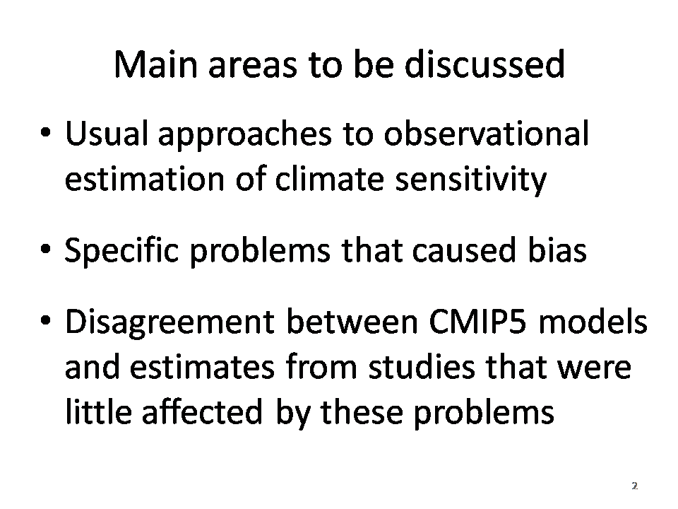
In this part I will cover the first bullet point and one of the major problems that cause bias in climate sensitivity estimates. In the second part I will deal with one or two other major problems and summarize the current position regarding observationally-based climate sensitivity estimation. In the final part I will deal with the third bullet point.
In a nutshell, I will argue that:
- Climate sensitivity is most reliably estimated from observed warming over the last ~150 years
- Most of the sensitivity estimates cited in the latest IPCC report had identifiable, severe problems
- Estimates from observational studies that are little affected by such problems indicate that climate sensitivity is substantially lower than in most global climate models
- Claims that the differences are due to substantial downwards bias in estimates from these observational studies have little support in observations.
Slide 3
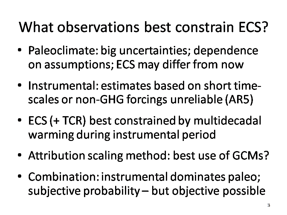
In many but not all current generation (CMIP5) AOGCMs, effective climate sensitivity estimates based on transient forced warming fall short of ECS, to an extent depending on the model, the estimation period, the forcing profile and the method used. It is unknown whether effective and equilibrium climate sensitivity differ much in the real world.
A shorter term measure of sensitivity, transient climate response (TCR) represents the increase in GMST over a 70 year period during which CO2 concentration increases at 1% p.a., thereby doubling. The focus at Ringberg 2015 was mainly on ECS, which can be related, at least approximately, to the physical concepts of (a) the effective radiative forcing (ERF) that a doubling of CO2 concentration produces and (b) the sum of the climate feedbacks to surface warming. Although TCR depends also on ocean heat uptake characteristics and is thus does not have a simple physical interpretation, it is more relevant than ECS to warming over this century.
The first three bullet points of Slide 3 reiterate what the IPCC fifth assessment WG1 report (AR5) said in Chapters 10 and 12 about palaeoclimate ECS estimates and those based on short timescales or non-greenhouse gas (GHG) forcings, and its implicit conclusion that estimates based on multidecadal warming during the instrumental period (since about 1850) were likely to prove most reliable and provide the narrowest uncertainty bounds.
ECS estimates based on multidecadal warming typically use simple or intermediate complexity climate models driven by estimated forcing timeseries, and measure how well simulated surface temperatures and ocean heat uptake compare with observations as model parameters are adjusted. Energy budget methods are also used. These involve deriving ECS and/or TCR directly from estimates changes in forcing and measured changes in GMST and ocean heat content, usually between decadal or longer periods at the start and end of the multidecadal analysis period. Alternatively, regression-based slope estimates are sometimes used.
Attribution scaling methods refers to the use of scaling factors (multiple regression coefficients) derived from detection and attribution analyses that match observed warming to the sum of scaled AOGCM responses to different categories of forcing, based on their differing spatiotemporal fingerprints. The derived scaling factor for warming attributable to GHG can then be used to estimate ECS and/or TCR, using a simple model. This hybrid method of observationally-estimating ECS and TCR appears to work better than the ‘PPE’ approach, which involves varying AOGCM model parameters.
Various studies have combined palaeoclimate and instrumental ECS estimates using subjective Bayesian methods. I do not believe that such methods are appropriate for ECS estimation, as the results are sensitive to the subjective choice of prior distribution. It is however possible to use objective methods – both Bayesian and frequentist – to combine probabilistic ECS estimates, provided that the estimates are independent – which palaeo and instrumental estimates are usually assumed to be. However, since palaeo ECS estimates are normally less precise than good instrumental ones, combination estimates are usually dominated by the underlying instrumental estimate.
Slide 4
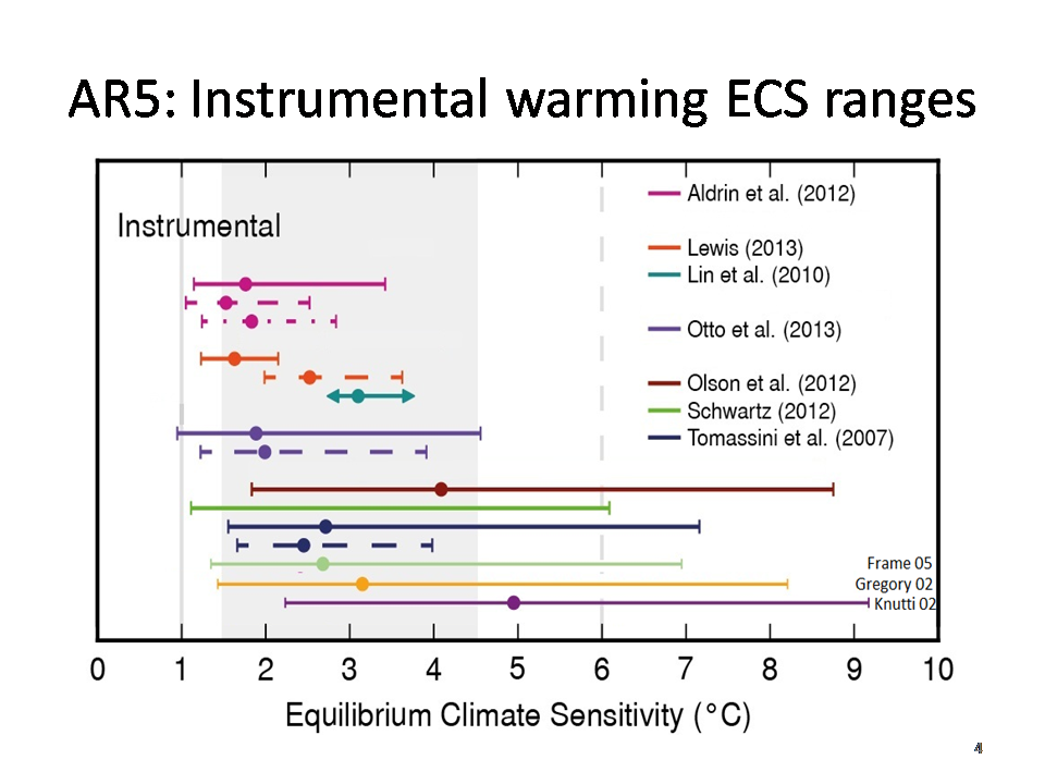
For the Lewis (2013) study, the dashed range should be ignored and the solid range widened to 1.0–3.0°C (with unchanged median) to reflect non-aerosol forcing uncertainty, as discussed in that paper.
Although the underlying forcing and temperature data should be quite similar in all these studies, the estimates vary greatly.
Slide 5
The relevant forcing concept here is ERF, denoted here by ΔF. AR5 defines it as follows: “ERF is the change in net TOA [top of atmosphere] downward radiative flux after allowing for atmospheric temperatures, water vapour and clouds to adjust, but with surface temperature or a portion of surface conditions unchanged.”
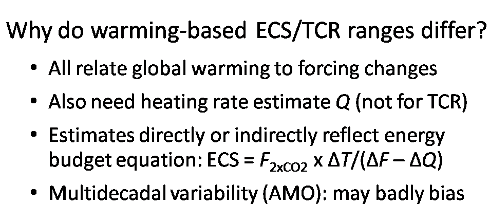
ΔT refers to the change in GMST resulting from a change in ERF, and ΔQ to a change in the planetary heating rate, mainly (>90%) reflected in ocean heat uptake.
Without using ocean heat content (OHC) data to estimate ΔQ, ECS tends to be ill-constrained.
ΔQ is not relevant to estimating TCR: the equivalent equation for generic TCR given in AR5 Chapter 10 is TCR = F2xCO2 ⨯ ΔT / ΔF.
Pre-2006 ECS studies almost all used the Levitus (2000) OHC data, which – due apparently to an uncorrected arithmetic error – gave substantially excessive values for ΔQ. Lin 2010 also used an excessive estimate for ΔQ, taken from the primarily model-based Hansen et al (2005) study. Moreover, many of the studies make no allowance for ΔQ being non-negligibly positive at the start of the instrumental period, as the Earth continued its recovery from the Little Ice Age. Gregory et al (2013) gives estimates of steric sea-level rise from 1860 on, derived from a naturally-forced model simulation starting in 850. Converting these to the planetary energy imbalance, and scaling down by 40% to allow for the model ECS of 3°C being high, gives ΔQ values of 0.15 W/m2 over 1860-1880 and 0.2 W/m2 from 1915-1960 (ΔQ being small in the intervening period due to high volcanism).
Multidecadal variability, represented by the quasi-periodic Atlantic Multidecadal Oscillation (AMO) in particular, means that the analysis period chosen is important. The AMO seems to be a genuine internal mode of variability, not as has been argued a forced pattern caused by anthropogenic aerosols.
The NOAA AMO index exhibits 60–70 year cycles over the instrumental period, peaking in the 1870s, around 1940, and in the 2000s. The AMO affects GMST, with a stronger influence in the northern hemisphere. As well as altering heat exchange between the ocean and atmosphere, the AMO also appears to modulate internal forcing through changing clouds – a little recognised point. As I will explain, the AMO can distort ECS estimation more seriously than its influence on GMST – of maybe ~0.2°C peak-to-peak – suggests.
Slide 6
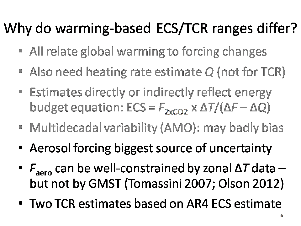
Uncertainty as to the change in aerosol forcing occurring during the instrumental period, ΔFaero, is the most important source of uncertainty in most ECS and TCR estimates based on multidecadal warming. Chapter 8 of AR5 gives a 1.8 W/m2 wide 5-95% range for ΔFaero over 1750–2011, about as large as the best estimate for (ΔF – ΔQ). The Lewis and Curry (2014) energy budget based study used the AR5 best estimate and uncertainty range for aerosol forcing (as well as other forcings), and hence its ECS and TCR estimates have 95% bounds that are much higher than their median values.
Otto et al (2013), although likewise using an energy budget method, used estimated forcings in CMIP5 AOGCMs (Forster et al 2013), which exhibit a narrower uncertainty range than AR5 gives, and adjusted their central value to reflect the difference between AOGCM and AR5 aerosol forcing estimates. Its resulting median estimate for TCR was accordingly almost identical to that in Lewis and Curry (2014), but its 95% bound based on the most recent data was lower.
It is possible to estimate ΔFaero with considerably less uncertainty than that stated in AR5, using “inverse methods” that infer ΔFaero from hemispherically- or zonally-resolved surface temperature data. This takes advantage of the latitudinally-inhomogeneous, northern hemisphere dominated, distribution of anthropogenic aerosol emissions, using a latitudinally-resolving model to estimate the spatial pattern of temperature changes at varying ΔFaero levels. Of the ECS studies featured in AR4 and AR5, Andronova and Schlesinger (2001), Forest et al (2002 and 2006), Liberdoni and Forest (2011/13), Ring, Schlesinger et al (2012), Aldrin et al (2012) and Lewis (2013) used this approach; so did Skeie et al (2014).
However, inverse estimates of ΔFaero are very unreliable if only GMST data is used. At a global level the evolution of ΔFaero and ΔFGHG is very highly correlated (r = 0.98 for the AR5 best estimate timeseries). Moreover, the diverge of the growth rates of the two series post the 1970s, when aerosol emissions flattened out, coincides and gets conflated with the AMO upswing.
Slide 7
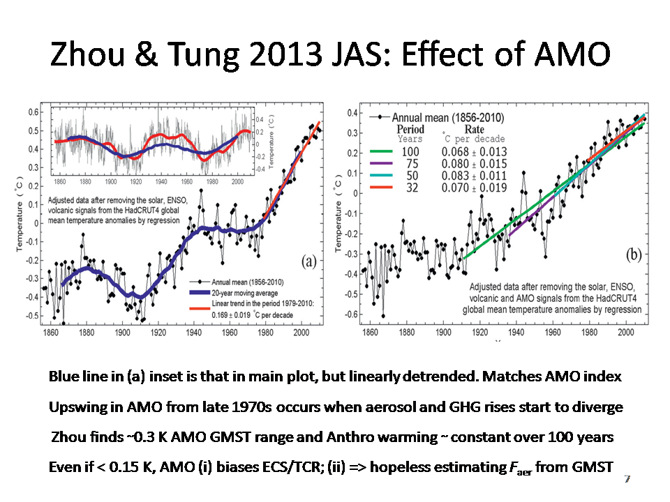
The AMO index smoothed pattern is shown by the red curve in the inset at the top of the LH panel of Slide 7, and can be seen to resemble the detrended GMST with shorter term natural signals removed (blue curve). The RH panel is not relevant to my argument, and can be ignored. Zhou and Tung may be overestimating the influence of the AMO on GMST (their range is in fact over 0.4 K, not 0.3 K as per the slide); Delsole et al (2011) estimate it to be about half as strong. However, even at one-quarter of the level shown it is enough to bias estimation of ΔFaero up by a factor of two or more, with an accompanying upwards bias of 20% or more in the estimate of warming attributable to GHG (and hence in TCR estimates; ECS estimates are even worse affected).
The problem is that a combination of a strongly negative estimate for ΔFaero, and a high estimate for ECS is able to mimic the effect on GMST caused by a factor (the AMO) not represented in the estimation model used. The slight fall in GMST between the 1940s and the early 1970s is matched by selecting a strongly growing negative ΔFaero that counters increasingly positive ΔFGHG, whilst the fast rise in GMST from the late 1970s on is matched by a high ECS (and hence high TCR), operating on a strong rise in ΔFGHG that is no longer countered by strengthening ΔFaero.
The ECS and TCR studies that use only the evolution of GMST (along with data pertaining to ΔQ) to estimate ΔFaero jointly with ECS therefore usually reach a much more negative estimate for ΔFaero, and a higher estimate for ECS, than studies that are able to estimate ΔFaero from the differential evolution of hemispherically- or zonally-resolved surface temperature data. Studies affected by this problem include, for ECS, Knutti et al (2002), Tomassini et al (2007) and Olson et al (2012) and, for TCR, Knutti & Tomassini 2008 and Padilla et al (2011).
Using hemispherically- or zonally-resolved temperature data to estimate aerosol forcing fails to avoid contamination by the AMO when the analysis period is insufficiently long. Many AR4 era ECS and TCR studies used the 20th century as their analysis period. The1900s started with the AMO low and ended with the AMO high. Gillett et al (2012) found that, despite its uses of spatiotemporal patterns, their detection and attribution study’s estimate of warming attributable to GHG was biased ~40% high when based on 1900s data compared to with when the longer 1851-2010 period was used. ECS studies affected by this problem include Gregory et al (2002), Frame et al (2005) and Allen et al (2009).The Stott and Forest (2007) TCR estimate is also affected.
The Gregory and Forster (2008) TCR estimate, while avoiding the AMO’s influence on aerosol forcing estimation, is significantly biased up by the AMO’s direct enhancement of the GMST trend over the short 1970–2006 analysis period used.
I will leave it there for Part 1; in Part 2 I will move on to problems with Bayesian approaches to climate sensitivity estimation.
Nicholas Lewis
References
Aldrin, M., M. Holden, P. Guttorp, R.B. Skeie, G. Myhre, and T.K. Berntsen, 2012. Bayesian estimation of climate sensitivity based on a simple climate model fitted to observations of hemispheric temperatures and global ocean heat content. Environmetrics;23: 253–271.
Andronova, N.G. and M.E. Schlesinger, 2001. Objective estimation of the probability density function for climate sensitivity. J. Geophys. Res.,106 (D19): 22605–22611.
DelSole, T., M. K. Tippett, and J. Shukla, 2011: A significant component of unforced multidecadal variability in the recent acceleration of global warming. J. Clim., 24, 909–926.
Forest, C.E., P.H. Stone, A.P. Sokolov, M.R. Allen and M.D. Webster, 2002.Quantifyinguncertainties in climate system properties with the use of recent climate observations. Science; 295: 113–117
Forest, C.E., P.H. Stone and A.P. Sokolov, 2006.EstimatedPDFs of climate system properties including natural and anthropogenic forcings. Geophys. Res. Lett., 33: L01705
Forster, P.M., T. Andrews, P. Good, J.M. Gregory, L.S. Jackson, and M. Zelinka, 2013. Evaluating adjusted forcing and model spread for historical and future scenarios in the CMIP5 generation of climate models. J. Geophys. Res., 118: 1139–1150.
Frame D.J., B.B..B. Booth, J.A. Kettleborough, D.A. Stainforth, J.M. Gregory, M. Collins and M.R. Allen, 2005.Constrainingclimateforecasts: The role of prior assumptions. Geophys. Res. Lett., 32, L09702Fyfe, J.C., N.P. Gillett, and F.W. Zwiers, 2013.Overestimatedglobal warming over the past 20 years. Nature Clim.Ch.; 3.9: 767–769.
Gillett NP, Arora VK, Flato GM, Scinocca JF, von Salzen K (2012) Improved constraints on 21st-century warming derived using 160 years of temperature observations. Geophys. Res. Lett., 39, L01704, doi:10.1029/2011GL050226.
Gregory, J.M., R.J. Stouffer, S.C.B. Raper, P.A. Stott, and N.A. Rayner, 2002. An observationally based estimate of the climate sensitivity. J. Clim.,15: 3117–3121.
Gregory, J. M., and P. M. Forster, 2008: Transient climate response estimated from radiative forcing and observed temperature change. J. Geophys. Res. Atmos., 113, D23105.
Knutti, R., T.F. Stocker, F. Joos, and G.-K. Plattner, 2002. Constraints on radiative forcing and future climate change from observations and climate model ensembles. Nature, 416: 719–723.
Knutti, R., and L. Tomassini, 2008: Constraints on the transient climate response from observed global temperature and ocean heat uptake. Geophys. Res. Lett., 35, L09701.
Levitus, S., J. Antonov, T. Boyer, and C Stephens, 2000. Warming of the world ocean, Science; 287: 5641.2225–2229.
Lewis, N., 2013. An objective Bayesian, improved approach for applying optimal fingerprint techniques to estimate climate sensitivity. J. Clim.,26: 7414–7429.
Lewis N, Curry JA (2014) The implications for climate sensitivity of AR5 forcing and heat uptake estimates. Clim. Dyn. DOI 10.1007/s00382-014-2342-y
Libardoni, A.G. and C. E. Forest, 2011. Sensitivity of distributions of climate system properties to the surface temperature dataset. Geophys. Res. Lett.; 38, L22705. Correction, 2013: doi:10.1002/grl.50480.
Lin, B., et al., 2010: Estimations of climate sensitivity based on top-of-atmosphere radiation imbalance. Atmos. Chem. Phys., 10: 1923–1930.
Meinshausen, M., et al., 2009: Greenhouse-gas emission targets for limiting global warming to 2 °C. Nature, 458, 1158–1162.
Olson, R., R. Sriver, M. Goes, N.M. Urban, H.D. Matthews, M. Haran, and K. Keller, 2012. A climate sensitivity estimate using Bayesian fusion of instrumental observations and an Earth System model. J. Geophys. Res. Atmos.,117: D04103.
Otto, A., et al., 2013. Energy budget constraints on climate response. Nature Geoscience, 6: 415–416.
Padilla, L. E., G. K. Vallis, and C. W. Rowley, 2011: Probabilistic estimates of transient climate sensitivity subject to uncertainty in forcing and natural variability. J. Clim., 24, 5521–5537.
Ring, M.J., D. Lindner, E.F. Cross, and M.E. Schlesinger, 2012. Causes of the global warming observed since the 19th century. Atmos. Clim. Sci., 2: 401–415.
Rogelj, J., M. Meinshausen, and R. Knutti, 2012: Global warming under old and new scenarios using IPCC climate sensitivity range estimates. Nature Clim. Change, 2, 248–253.
Schwartz, S.E., 2012. Determination of Earth’s transient and equilibrium climate sensitivities from observations over the twentieth century: Strong dependence on assumed forcing. Surv.Geophys., 33: 745–777.
Tomassini, L., P. Reichert, R. Knutti, T.F. Stocker, and M.E. Borsuk, 2007. Robust Bayesian uncertainty analysis of climate system properties using Markov chain Monte Carlo methods. J. Clim., 20: 1239–1254.
Zhou, J., and K.-K. Tung, 2013. Deducing multidecadal anthropogenic global warming trends using multiple regression analysis. J. Atmos. Sci., 70, 3–8.
Leave A Comment