Originally posted on Apr 13, 2015 – 5:02 PM at Climate Audit
In Part 1 I introduced the talk I gave at Ringberg 2015, explained why it focussed on estimation based on warming over the instrumental period, and covered problems relating to aerosol forcing and bias caused by the influence of the AMO. I now move on to problems arising when Bayesian probabilistic approaches are used, and then summarize the state of instrumental period warming, observationally-based climate sensitivity estimation as I see it. I explained in Part 1 why other approaches to estimating ECS appear to be less reliable.
Slide 8
The AR4 report gave probability density functions (PDFs) for all the ECS estimates it presented, and AR5 did so for most of them. PDFs for unknown parameters are a Bayesian probabilistic concept. Under Bayes’ theorem – a variant on the conditional probability lemma – one starts by choosing a prior PDF for the unknown parameter, then multiplies it by the relative probability of having obtained the actual observations at each value of the parameter (the likelihood function), thus obtaining, upon normalising the result to unit total probability, a posterior PDF representing the new estimate of the parameter.
The posterior PDF melds any existing information about the parameter from the prior with information provided by the observations. If multiple parameters are being estimated, a joint prior and a joint likelihood function are required, and marginal posterior PDFs for individual parameters are obtained by integrating out the other parameters from the joint posterior PDF.
Uncertainty ranges derived from percentage points of the integral of the posterior PDF, the posterior cumulative probability distribution (CDF), are known as credible intervals (CrI). The frequentist statistical approach instead gives confidence intervals (CIs), which are conceptually different from CrIs. In general, a Bayesian CrI cannot be exactly equivalent to a frequentist CI no matter what prior is selected. However, for some standard cases they can be the same, and it is typically possible to derive a prior (a probability matching prior) which results in CrIs being close to the corresponding CIs. That is critical if assertions based on a Bayesian CrI are to be true with the promised reliability.
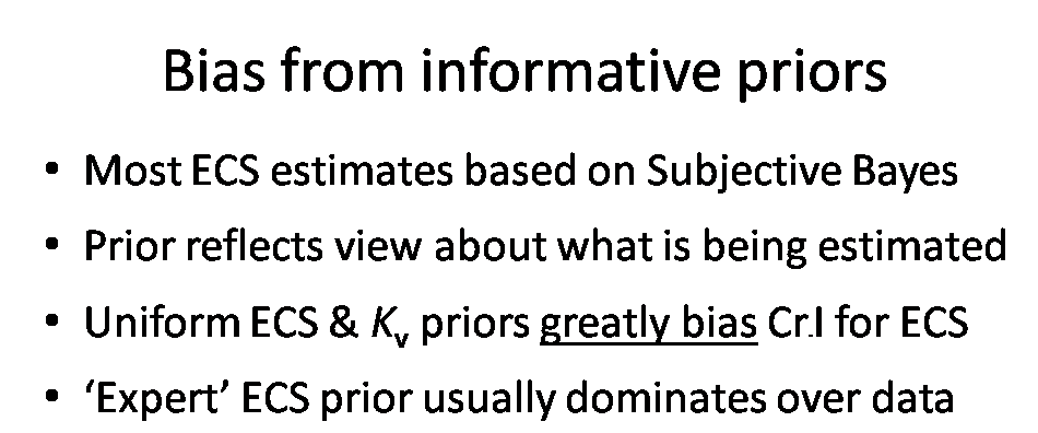
Almost all the PDFs for ECS presented in AR4 and AR5 used a ‘subjective Bayesian’ approach, under which the prior is selected to represent the investigator’s views as to how likely it is the parameter has each possible value. A judgemental or elicited ‘expert prior’ that typically has a peaked distribution indicating a most likely value may be used. Or the prior may be a diffuse, typically uniform, distribution spread over a wide range, intended to convey ignorance and/or with a view to letting the data dominate the posterior PDF. Unfortunately, the fact that a prior is diffuse does not in fact mean that it conveys ignorance or lets the data dominate parameter inference.
AR4 stated that all its PDFs for ECS were presented on a uniform-in-ECS prior basis, although the AR4 authors were mistaken in two cases. In AR5, most ECS PDFs were derived using either uniform or expert priors for ECS (and for other key unknown parameters being estimated alongside ECS).
When the data is weak (is limited and uncertainty is high) the prior can have a major influence on the posterior PDF. Unlike in many areas of physics, that is the situation in climate science, certainly so far as ECS and TCR estimation is concerned. Moreover, the relationships between the principal observable variables (changes in atmospheric and ocean temperatures) and the parameters being estimated – which typically also include ocean effective vertical diffusivity (Kv) when ECS is the target parameter – are highly non-linear.
In these circumstances, use of uniform priors for ECS and Kv (or its square root) greatly biases posterior PDFs for ECS, raising their medians and fattening their upper tails. On the other hand, use of an expert prior typically results in the posterior PDF resembling the prior more than it reflects the data.
Slide 9
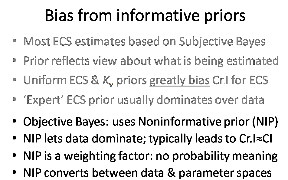
Some studies used, sometimes without realising it, the alternative ‘objective Bayesian’ approach, under which a mathematically-derived noninformative prior is used. Although in most cases it is impossible to formulate a prior that has no influence at all on the posterior PDF, the form of a noninformative prior is calculated so that it allows even weak data to dominate the posterior PDF for the parameter being estimated. Noninformative priors are typically judged by how good the probability-matching properties of the resulting posterior PDFs are.
Noninformative priors do not represent how likely the parameter is to take any particular value and they have no probabilistic interpretation. Noninformative priors are simply weight functions that convert data-based likelihoods into parameter posterior PDFs with desirable characteristics, typically as regards probability matching. This is heresy so far as the currently-dominant Subjective Bayesian school is concerned. In typical ECS and TCR estimation cases, noninformative priors are best regarded as conversion factors between data and parameter spaces.
For readers wanting insight as to why noninformative priors have no probability meaning, contrary to the standard interpretation of Bayes’ theorem, and regarding problems with Bayesian methods generally, I recommend Professor Don Fraser’s writings, perhaps starting with this paper.
The Lewis (2013) and Lewis (2014) studies employed avowedly objective Bayesian approaches, involving noninformative priors. The Andronova and Schlesinger (2001), Gregory et al (2002), Otto et al (2013), and Lewis & Curry (2014) studies all used sampling methods that equated to an objective Bayesian approach. Studies using profile likelihood methods, a frequentist approach that yields approximate CIs, also achieve objective estimation (Allen et al 2009, Lewis 2014).
Slide 10
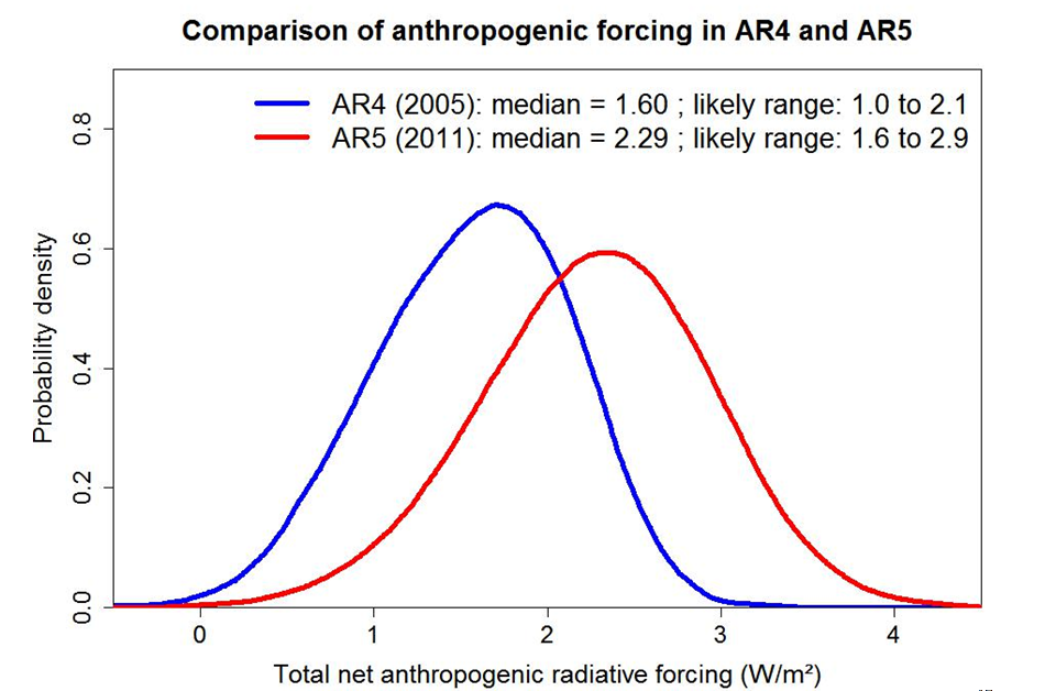
I will illustrate the effect of using a uniform prior for TCR estimation, that being a simpler case than ECS estimation. Slide 10 shows estimated distributions from AR4 and AR5 for anthropogenic forcing, up to respectively 2005 and 2011. These are Bayesian posterior PDFs. They are derived by sampling from estimated uncertainty distributions for each forcing component, and I will assume for the present purposes that they can be considered to be objective.
Slide 11
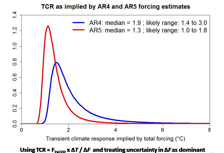
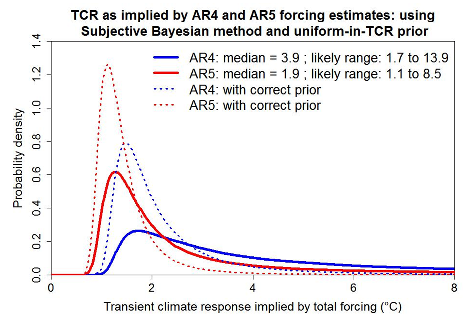
Slide 11 shows posterior PDFs for TCR derived from the AR4 and AR5 PDFs for anthropogenic forcing, ΔF, by making certain simplifying approximations. I have assumed that the generic-TCR formula given in AR5 holds; that uncertainty in the GMST rise attributable to anthropogenic forcing, ΔT , and in F2xCO2, the forcing from a doubling of CO2, is sufficiently small relative to uncertainty in ΔF to be ignored; and that in both cases ΔT = 0.8°C and F2xCO2 = 3.71 W/m2.
On this basis, posterior PDFs for TCR follow from a transformation of variables approach. One simply changes variable from ΔF to TCR (the other factors in the equation being assumed constant). The PDF for TCR at any value TCRa therefore equals the PDF for ΔF at ΔF = F2xCO2 ⨯ ΔT / TCRa , multiplied by the standard Jacobian factor: the absolute derivative of ΔF with respect to TCR at TCRa. That factor equals, up to proportionality, 1/TCR2.
Slide 12
Suppose one regards the posterior PDFs for ΔF as having been derived using uniform priors. This is accurate in so far as components of ΔF have symmetrical uncertainty distributions, but overall it is only an approximation since the most uncertain component, aerosol forcing, is assumed to have an asymmetrical distribution. However, the AR4 and AR5 PDFs for ΔF are not greatly asymmetrical.
On the basis that the posterior PDFs for ΔF correspond to the normalised product of a uniform prior for ΔF and a likelihood function, the PDFs for TCR derived in slide 11 correspond to the normalised product of the same likelihood function (now expressed in terms of TCR) and a prior having the form 1/TCR2. Unlike PDFs, likelihood functions do not depend on which variable that they are expressed in terms of. That is because, unlike a PDF, a likelihood function represents a density for the observed data, not for the variable that it is expressed in terms of.
The solid lines in slide 12 show, on the foregoing basis, what the effect is on the AR4- and AR5-forcing based posterior PDFs for TCR of substituting a uniform-in-TCR prior for the mathematically correct 1/TCR2 prior applying in slide 11 (the PDFs from which are shown dotted). The median (50% probability point), which is the appropriate best estimate to use for a skewed distribution, increases substantially, doubling in the AR4 case. The top of the 17–83% ‘likely’ range more than quadruples in both cases. The distortion for ECS estimates would be even larger.
Slide 12a
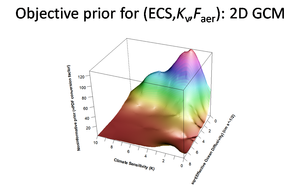
I cut slide 12a out of my talk to shorten it. It shows the computed joint noninformative prior for ECS and sqrt(Kv) from Lewis (2013). Noninformative priors can be quite complex in form when multiple parameters are involved.
Ignore the irregularities and the rise in the front RH corner, which are caused by model noise. Note how steeply the prior falls with sqrt(Kv), which is lowest at the rear, particularly at high ECS levels (towards the left). The value of the prior reflects how informative the data is about the parameters at each point in parameter space. The plot is probability-averaged over all values for aerosol forcing, which was also being estimated. I believe the fact that aerosol forcing is being estimated accounts for the turndown in the prior at low ECS values; when ECS is very low temperaturs change little and the data conveys less information about aerosol forcing.
Slide 13
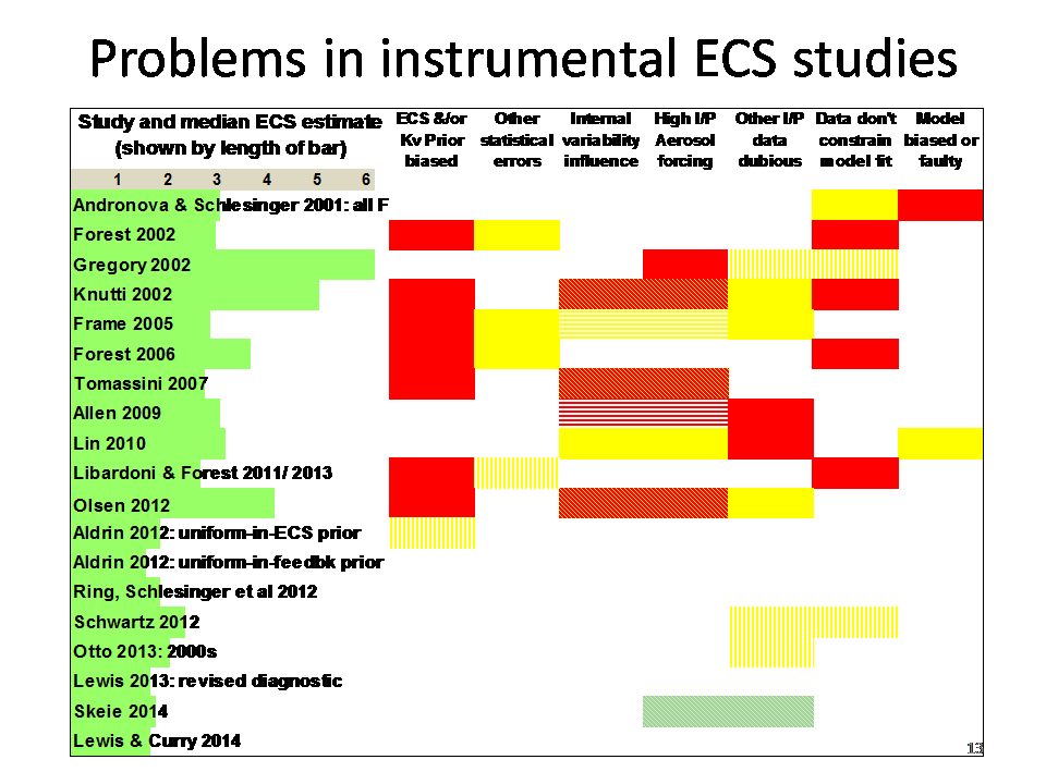
Slide 13 summarises serious problems in instrumental period warming based ECS studies, ordered by year of publication, breaking problems down between seven factors. Median ECS estimates are shown by the green bars at the left.
Blank rectangles imply no significant problem in the area concerned; solid yellow or red rectangles signify respectively a significant and a serious problem; a rectangle with vertical yellow bars, which may look like solid pale yellow, indicates a minor problem.
Red/yellow diagonal bars (may look like a solid orange shade of red) in rectangles across ‘Internal variability influence’ and ‘High input Aerosol forcing’ mean that, due to use of global-only data, internal variability (the AMO) has led to an overly negative estimate for aerosol forcing within the study concerned, and hence to an overestimate of ECS. Yellow or red horizontal bars across those factors for the Frame et al (2005) and Allen et al (2009) studies mean that internal variability appears to have caused respectively significant or serious misestimation of aerosol forcing in the detection and attribution study that was the source of the (GHG-attributable) warming estimate used by the ECS study involved, and hence to upwards bias in that estimate (reflected in a yellow or red rectangle for ‘Other input data dubious’).
The blue/yellow horizontal bar across ‘High input Aerosol forcing’ and ‘Other input data dubious’ for the Skeie et al (2014) study mean that problems in these two areas largely cancelled. Skeie’s method estimated aerosol forcing using hemispherically-resolved model-simulation and observational data. An extremely negative prior for aerosol forcing was used, overlapping so little with the observational data-based likelihood function that the posterior estimate was biased significantly negative. However, the simultaneous use of three ocean heat content observational datasets appears to have led to the negatively biased aerosol forcing being reflected in lower modelled than observed NH warming rather than a higher ECS estimate.
The ‘Data don’t constrain model fit’ red entries for the Forest studies are because, from my experience, warming over the model-simulation run using the claimed best-fit parameter values is substantially greater than per the observational dataset. The same entry for Knutti et al (2002) is because a very weak, pass/fail, statistical test was used in that study.
The ‘Model biased or faulty’ red rectangle for Andronova and Schlesinger (2001) reflects a simple coding error that appears to have significantly biased up its ECS estimation: see Table 3 in Ring et al (2012).
A more detailed analysis of problems with individual ECS studies is available here.
To summarise: all pre-2012 instrumental-period-warming studies had one or more serious problems, and their median ECS estimates varied widely. Most studies from 2012 on do not appear to have serious problems, and their estimates agree quite closely. (The Schwartz 2012 study’s estimate was a composite of five estimates based on different forcing series, the highest ECS estimate comes from a poor quality regression obtained from one of the series.)
Slide 14
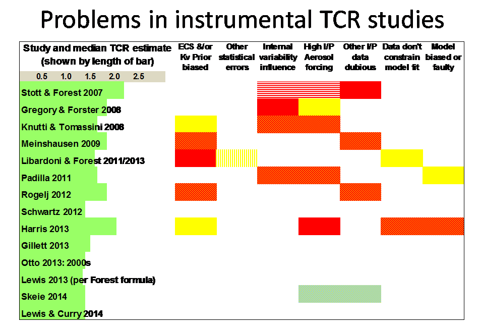
Slide 14 gives similar information to slide 13, but for TCR rather than ECS studies. As for ECS, all pre-2012 studies had one or more serious problems that make their TCR estimates unreliable, whilst most later studies do not have serious problems apparent and their median TCR estimates are quite close to one another.
Rogelj et al (2012)’s high TCR estimate is not genuinely observationally-based; it is derived from an ECS distribution chosen to match the AR4 best estimate and ‘likely’ range for ECS; the same goes for the Meinshausen et al (2009) estimate. The reason for the high TCR estimate from Harris et al (2013) is shown in the next slide.
A more detailed analysis of problems with individual TCR studies is available here.
Slide 14a
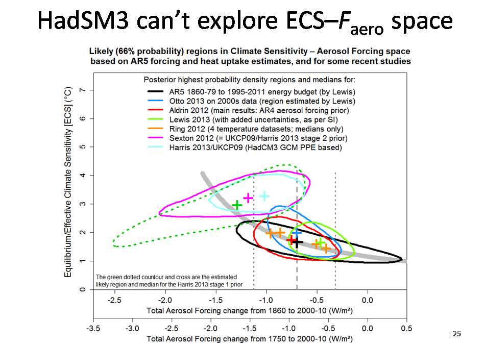
This slide came later in my talk, but rather than defer it to Part 3 I have moved it here as it relates to a PPE (perturbed physics/parameter ensemble) study, Harris et al (2013), mentioned in the previous slide. Although this slide considers ECS estimates, the conclusions reached imply that the Harris et al TCR estimate shown in the previous slide is seriously biased up relative to what observations imply.
The plot is of joint distributions for aerosol forcing and ECS; the solid contours enclose ‘likely’ regions, of highest posterior probability density, containing 66% of total probability. Median estimates are shown by crosses; the four Ring et al (2012) estimates based on different surface temperature datasets are shown separately. The black contour is very close to that for Lewis and Curry (2014).
The grey dashed (dotted) vertical lines show the AR5 median estimate and ‘likely’ range for aerosol forcing, expressed both from 1750 (preindustrial) and from 1860; aerosol forcing in GCMs is normally estimated as the change between 1850 or 1860 and 2000 or 2005. The thick grey curve shows how one might expect the median estimate for ECS using an energy budget approach, based on AR5 non-aerosol forcing best estimates and a realistic estimate for ocean heat uptake, to vary with the estimate used for aerosol forcing.
The median estimates from the studies not using GCMs cluster around the thick grey curve, and their likely regions are orientated along it: under an energy budget or similar model, high ECS estimates are associated with strongly negative aerosol forcing estimates. But the likely regions for the Harris study are orientated very differently, with less negative aerosol forcing being associated with higher, not lower, ECS. Its estimated prior distribution ‘likely’ region (dotted green contour) barely overlaps the posterior regions of the other studies: the study simply does not explore the region of low to moderately negative aerosol forcing, low to moderate ECS which the other studies indicate observations best support. It appears that the HadCM3/SM3 model has structural rigidities that make it unable to explore this region no matter how its key parameters are varied. So it is unsurprising that the Harris et al (2013) estimates for ECS, and hence also for TCR, are high: they cannot be regarded as genuinely observationally-based.
Further information on the problems with the Harris et al (2013) study is available here: see Box 1.
Slide 15
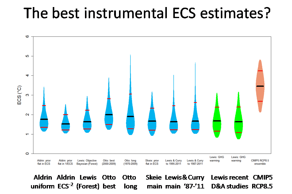
This slide shows what I regard as the least-flawed ECS estimates based on observed warming over the instrumental period, and compares them with ECS values exhibited by the RCP8.5 simulation ensemble of CMIP5 models. I should arguably have included the Schwartz (2012) and Masters (2014) estimates, but I have some concerns about the GCM-derived forcing estimates they use.
The violins span 5–95% ranges; their widths indicate how PDF values vary with ECS. Black lines show medians, red lines span 17–83% ‘likely’ ranges. Published estimates based directly on observed warming are shown in blue. Unpublished estimates of mine based on warming attributable to greenhouse gases inferred by two recent detection and attribution studies are shown in green. CMIP5 models are shown in salmon.
The observational ECS estimates have broadly similar medians and ‘likely’ ranges, all of which are far below the corresponding values for the CMIP5 models.
The ‘Aldrin ECS-2‘ violin is for its estimate that uses a uniform prior for 1/ECS, which equates to a ECS-2 prior for ECS. I believe that to be much closer to a noninformative prior than is the uniform-in-ECS prior used for the main Aldrin et al (2012) results. The Lewis (Forest) estimate is based on the Lewis (2013) preferred main ECS estimate with added non-aerosol forcing uncertainty, as shown in the study’s supplemental information.
Slide 16
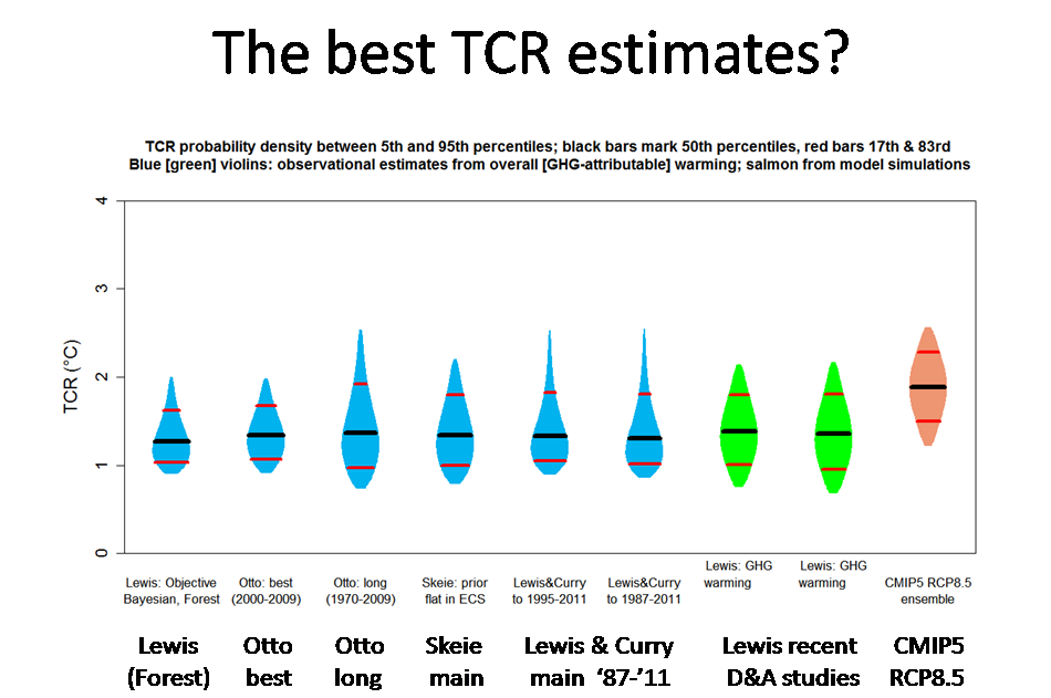
This slide is like the previous one, but relates to TCR not ECS.
As for ECS, the observational TCR estimates have broadly similar medians and ‘likely’ ranges, all of which are well below the corresponding values for the CMIP5 models.
The Schwartz (2012) TCR estimate, which has been omitted for no good reason, has a median of 1.33°C and a 5–95% range of 0.83–2.0°C.
The Lewis (Forest) estimate uses the same formula as in Libardoni and Forest (2011), which also uses the MIT 2D GCM, to derive model TCR from combinations of model ECS and Kv values.
Slide 17
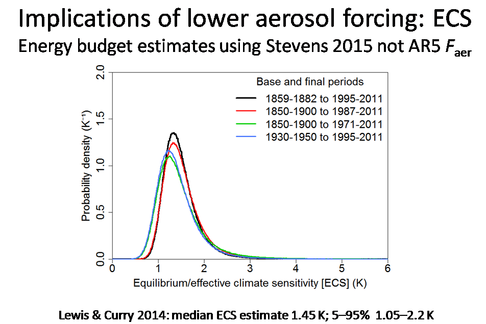
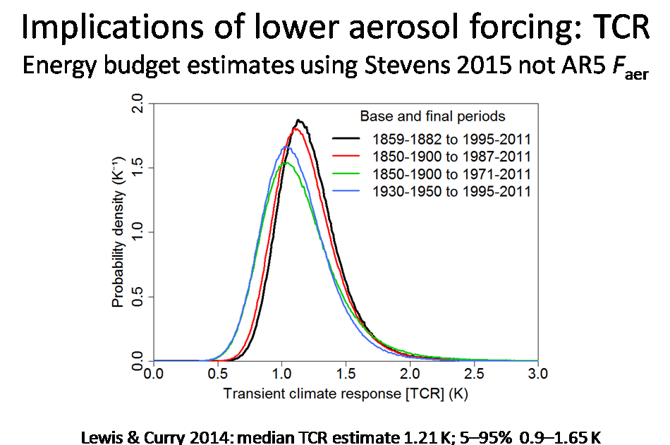
The main cause of long tails in ECS and TCR studies based on observed multidecadal warming is uncertainty as to the strength of aerosol forcing (Faer). I’ll end this part with a pair of slides that show how well constrained the Lewis and Curry (2014) energy-budget main ECS and TCR estimates would be if they were recalculated using the distribution for aerosol forcing implicit in Bjorn Stevens’ recent study instead of the wide AR5 aerosol forcing distribution. (For some reason these slides appear much later, out of order, in the PDF version of my slides on the Ringberg 2015 website.)
The median ECS estimate reduces modestly from 1.64°C to 1.45°C, but the 95% uncertainty bound falls dramatically, from 4.05°C to 2.2°C.
Slide 18
The picture is similar for TCR, although somewhat less dramatic. The median TCR estimate reduces modestly from 1.33°C to 1.21°C, but the 95% uncertainty bound falls much more, from 2.50°C to 1.65°C.
Nicholas Lewis
Additional references
Allen MR, Frame DJ, Huntingford C, Jones CD, Lowe JA, Meinshausen M, Meinshausen N (2009) Warming caused by cumulative carbon emissions towards the trillionth tonne. Nature, 458, 1163–6.
Frame DJ, Booth BBB, Kettleborough JA, Stainforth DA, Gregory JM, Collins M, Allen MR (2005) Constraining climate forecasts: The role of prior assumptions. Geophys. Res. Lett., 32, L09702, doi:10.1029/2004GL022241.
Harris, G.R., D.M.H. Sexton, B.B.B. Booth, M. Collins, and J.M. Murphy, 2013. Probabilistic projections of transient climate change. Clim. Dynam., doi:10.1007/s00382–012–1647-y.
Lewis N (2014) Objective Inference for Climate Parameters: Bayesian, Transformation-of-Variables, and Profile Likelihood Approaches. J. Climate, 27, 7270-7284.
Masters T (2014) Observational estimate of climate sensitivity from changes in the rate of ocean heat uptake and comparison to CMIP5 models. Clim Dynam 42:2173-2181 DOI 101007/s00382-013-1770-4
Sexton, D.M. H., J.M. Murphy, M. Collins, and M.J. Webb, 2012. Multivariate probabilistic rojections using imperfect climate models part I: outline of methodology. Clim. Dynam., 38: 2513–2542.
Stevens, B. Rethinking the lower bound on aerosol radiative forcing. In press, J.Clim (2015) doi: http://dx.doi.org/10.1175/JCLI-D-14-00656.1
Leave A Comment