Originally a guest post on Jan 8, 2016 – 4:42 PM at Climate Audit
Note: This is a long article: a summary is available here.
Introduction
In a recent paper[1], NASA scientists led by Kate Marvel and Gavin Schmidt derive the global mean surface temperature (GMST) response of the GISS-E2-R climate model to different types of forcing. They do this by simulations over the historical period (1850–2005) driven by individual forcings, and by all forcings together, the latter referred to as the ‘Historical’ simulation.
They assert that their results imply that estimates of the transient climate response (TCR) and equilibrium climate sensitivity (ECS) derived from recent observations are biased low.
Marvel et al. use the GISS-E2-R historical period simulation responses to revise estimates of the transient climate response (TCR) and equilibrium climate sensitivity (ECS) from three observationally-based studies: Otto et al. 2013, Lewis and Curry 2014 and Shindell 2014. Their revisions give figures that are substantially higher than in the original studies. Remarkably, the Marvel et al. reworked observational estimates for TCR and ECS are, taking the averages for the three studies, substantially higher than the equivalent figures for the GISS-E2-R model itself, despite the model exhibiting faster warming than the real climate system. Not only is the GMST increase simulated by GISS-E2-R is higher than that observed, but the ocean heat uptake rate is well above the observed level.[2] No explanation is given for this surprising result.
The press release for the paper quotes Kate Marvel as follows:
‘Take sulfate aerosols, which are created from burning fossil fuels and contribute to atmospheric cooling,’ she said. ‘They are more or less confined to the northern hemisphere, where most of us live and emit pollution. There’s more land in the northern hemisphere, and land reacts quicker than the ocean does to these atmospheric changes.’
and continues by saying:
‘Because earlier studies do not account for what amounts to a net cooling effect for parts of the northern hemisphere, predictions for TCR and ECS have been lower than they should be.’
However, this is not true when the effective radiative forcing (ERF) measure of aerosol forcing – preferred by IPCC AR5 and used in the observational studies Marvel et al. criticises – is employed. When calculated correctly using Marvel et al.’s data, bases and assumptions, aerosol ERF had a transient efficacy of 0.97 – almost the same as the 0.95 for GHG forcing and 1.00 for CO2 forcing. This result is in line with the findings in Hansen 2005.This implies that aerosol forcing has had almost the same effect on GMST since 1850, relative to its ERF, as did CO2 and GHG forcing. Its concentration in the northern hemisphere did not lead to a greater cooling effect globally since 1850.
Studies like Marvel et al. can be valuable in showing the effects of differing forcing agents in climate models, which – if similar across climate models – may provide a guide to their effects in the real climate system. Unfortunately, I believe that the Marvel et al. results are substantially inaccurate and misleading. Its conclusions are therefore unfounded. But, as with any single-model study, even were its results unimpeachable they would reflect the behaviour of the particular model involved, which may be very different from that of other models and, more importantly, from that of the real climate system.
Background
It is known that an equal radiative forcing caused by different agents may have a greater or lesser effect on GMST. That is to say, different types of forcing may have different ‘efficacies’. The efficacy of a forcing is defined as its effect on GMST relative to that of the same amount of forcing by CO2. The efficacy of CO2 forcing is therefore one. This definition is reasonable: CO2 is the dominant greenhouse gas and TCR and ECS are measures of the GMST response – respectively after 70 years of linearly increasing forcing, and after the ocean reaches equilibrium – to a doubling of CO2 concentration. The forcing–efficacy framework, to be useful, requires that GMST response scales linearly with forcing and that the GMST response to a mixture of different forcings equals the sum of the responses to the constituent individual forcings. Both these assumptions typically hold quite well in general circulation models (GCMs).
A seminal paper[3] lead authored by James Hansen of GISS (henceforth Hansen 2005), based on simulations by a previous version of the GISS GCM, Model E, estimated efficacies for different forcing agents. Hansen 2005, a commendably thorough paper, advanced climate science and helped pave the way for the use of effective radiative forcing (ERF) in IPCC AR5. Hansen 2005 derived efficacies in terms of both the instantaneous radiative flux change at the tropopause (iRF or Fi) and the flux change after the stratosphere has adjusted to the forcing (RF or Fa). RF is the same whether measured at the tropopause or the top-of-atmosphere (TOA). Hansen also derived efficacies relative to Fs, the TOA flux change with sea surface temperature (SST) held fixed, and Fs*, an approximation to Fs derived by regressing TOA flux on GMST following a step change in forcing, in a so-called Gregory plot, in this case for 10–30 years. Hansen’s Fs was adjusted for the change in land surface temperatures that occurs when forcing is changed but SST is held fixed.
Section 8.1 of AR5[4] gives a useful introduction to radiative forcing in its different variants. It defines ERF similarly to Hansen’s Fs, but with no adjustment made for the change in land temperature (which is modest when SST is fixed), and notes that ERF can also be estimated by regression, as for Fs*. The ERF, Fs and Fs* measures allow for the troposphere to adjust to the imposed forcing, as well as the stratosphere.
Hansen 2005 found that although when iRF was used to measure forcing, the efficacy of some forcing agents differed substantially from one, when either Fs and Fs* were used efficacies were close to one for almost all types of forcing investigated.
Further details of Hansen 2005’s findings, and information on relevant other studies are given in Appendix A.
Marvel et al.’s investigation of forcing efficacies
Marvel et al. used the newer E2-R version of the GISS model to carry out single-forcing simulations similar to those in Hansen 2005. However the set of simulations was more limited in scope and forcings were made to follow their estimated historical evolution from 1850 to 2005 rather than being imposed in full at the start of the simulation.
Forcings, in iRF terms, were derived each year by radiation-only calculations, with the forcing agent evolving but all other variables held at preindustrial (1850) values. ERFs were estimated only for the year 2000, from simulations with the then level of the forcing agent concerned and only SSTs fixed at 1850 values. Equilibrium and transient efficacies, and TCR and ECS estimates, were derived by comparing the historical GMST response (ΔT) with the causative forcing change (ΔF) respectively with and without the associated change in ocean heat uptake rate (ΔQ) deducted. The decadal mean ΔT, ΔF and ΔF−ΔQ values used are all anomalies relative to drift-adjusted quasi-equilibrium preindustrial control runs, from which these simulations were spawned in 1850. The mean ΔT and ΔQ values from an ensemble of five runs were used.
Specifically, the relationships between decadal means of ΔT and ΔF (for TCR) or ΔF − ΔQ (for ECS) in each forced simulation are used to produce separate estimates of GISS-E2-R’s TCR and ECS for each forcing agent, according to the energy budget equations:[5]
![]() where F2xCO2 is the forcing from a doubling of CO2 concentration. For ERF the ratios are simply quotients based on 1996–2005 values. For iRF, where values for all decades are available, the quotients that Marvel et al. use are the slopes of the best-fit lines when regressing ΔT using 1906–15 to 1996–2005 values. Marvel et al. calculate the transient (equilibrium) efficacy for each forcing as the ratio of the TCR (ECS) estimate it gives rise to divided by the actual, CO2 forced, values for GISS-E2-R, being 1.4°C for TCR and 2.3°C for ECS. Hansen 2005 instead derived transient efficacies (not equilibrium efficacies as stated by Marvel et al.) by directly comparing the ΔT/ΔF ratio for each forcing agent with that for CO2, in simulations with identical forcing time-profiles.
where F2xCO2 is the forcing from a doubling of CO2 concentration. For ERF the ratios are simply quotients based on 1996–2005 values. For iRF, where values for all decades are available, the quotients that Marvel et al. use are the slopes of the best-fit lines when regressing ΔT using 1906–15 to 1996–2005 values. Marvel et al. calculate the transient (equilibrium) efficacy for each forcing as the ratio of the TCR (ECS) estimate it gives rise to divided by the actual, CO2 forced, values for GISS-E2-R, being 1.4°C for TCR and 2.3°C for ECS. Hansen 2005 instead derived transient efficacies (not equilibrium efficacies as stated by Marvel et al.) by directly comparing the ΔT/ΔF ratio for each forcing agent with that for CO2, in simulations with identical forcing time-profiles.
In the ECS energy budget equation, ΔQ should be the TOA radiative imbalance (ΔN); Marvel et al. use the rate of ocean heat uptake (OHU) as an approximation to ΔN.
Marvel et al. state that in these equations F2xCO2 is taken as having an iRF of 4.1 W/m2; the ERF value used is not stated. Having derived efficacies for individual forcing agents, they then use them to re-estimate climate sensitivity from observed historical warming, using data for three previous studies and arriving at higher estimates than in those studies.
Figure 1 reproduces Figure 1a of Marvel et al., which shows the relationship in GISS-E2-R between changes ΔT in simulated GMST and ΔF in forcing, for six individual forcing agents as they are estimated to have evolved since 1850 and for the Historical simulations (all-forcings together, 6 runs). The forcing agents are long-lived greenhouse gases (GHG), anthropogenic aerosols (AA), land-use changes (LU), ozone (Oz), solar (SI) and volcanoes (VI). The filled circles are with forcing measured by iRF, and show means for decades ending from 1906–15 to 1996–2005. The open circles are for 1996–2005 mean GMST changes with forcing measured by ERF in 2000; the ΔT values are the same as for iRF.
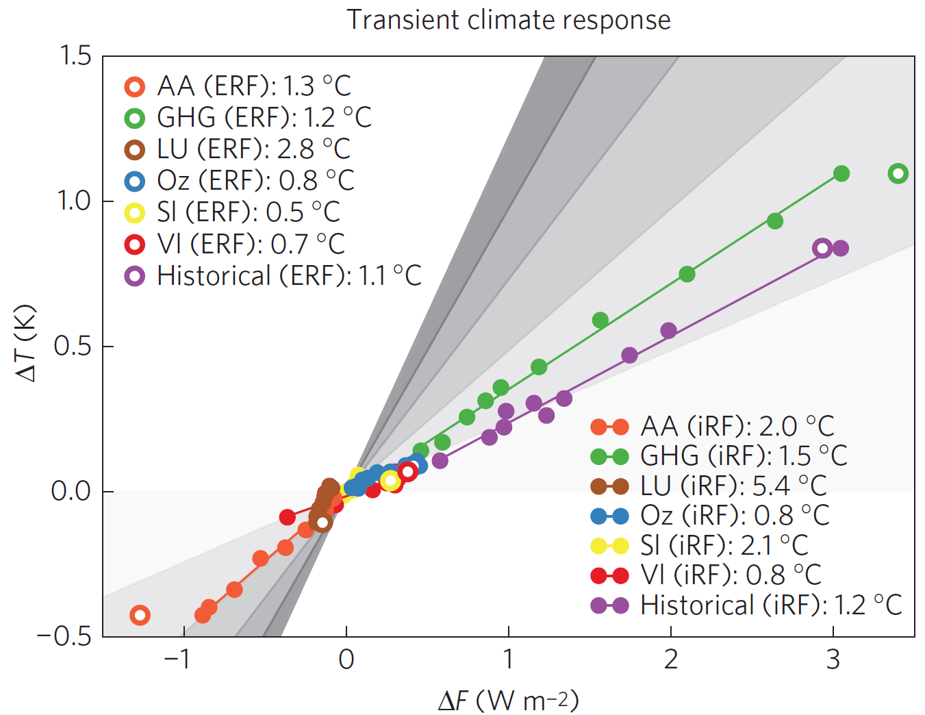 Figure 1: Reproduction of Figure 1a of Marvel et al.
Figure 2 reproduces Figure 1b of Marvel et al. It differs from Figure 1 only in that the x-axis shows ΔF−ΔQ rather than ΔF, as here equilibrium rather than transient sensitivity (and hence efficacy) is being estimated.
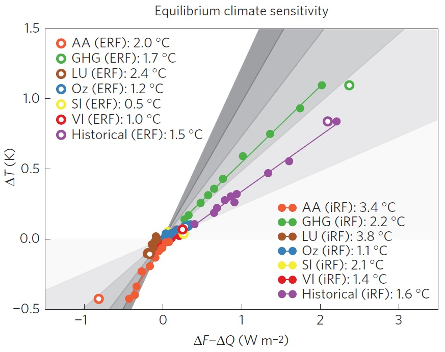 Figure 2: Reproduction of Figure 1b of Marvel et al.
Fundamental problems with Marvel et al.’s estimation of forcing efficacies, TCR and ECS
There are at least six fundamental problems with Marvel et al. estimation methodology and its implementation, apart from the fact that the estimates relate to the behaviour of GISS-E2-R model, not the real world.
- What is primarily relevant for observational estimates of climate sensitivity based on changes over the historical period is how much forcing and warming recent levels of different forcing agents generate in today’s climate state, relative to the preindustrial (1850) state of affairs. By contrast, Marvel et al. estimate the forcing and resulting warming produced in the preindustrial climate system when it is altered in one respect only: the concentration of a single forcing agent. For non-GHG forcing agents, this leaves the climate in a near preindustrial, or colder climate state, not close to today’s climate state. In GISS-E2-R these two situations can, at least for certain agents, give rise to very different levels of forcing, whether or not they do so in reality; it is unclear to what extent the GMST responses in the two cases will reflect their different measured forcings.For example, in GISS-E2-R the 2000 level of anthropogenic aerosol loading produces direct aerosol TOA radiative forcing of –0.40 W/m2 in the 2000 climate, but zero forcing in the 1850 climate.[6] Also, ozone iRF forcing in GISS-E2-R differs when the climate state is allowed to evolve as in the all-forcings simulation: 0.28 W/m2 in 2000 versus 0.45 W/m2 per Marvel et al.’s value based on an approximately preindustrial climate state.21 This shows that for some forcing agents Marvel et al.’s methodology does not correctly quantify forcing in GISS-E2-R for recent decades of the Historical simulation, making its related efficacy and sensitivity estimates very doubtful.
- The energy budget equation for ECS actually estimates effective climate sensitivity for the timescale over which changes are measured, which only equals equilibrium climate sensitivity if feedbacks do not vary with time.[7] However, effective climate sensitivity in GISS-E2-R increases with time since the forcing was applied, as in many GCMs. Efficacy is defined as a forcing agent’s effect on GMST relative to that of the same forcing from CO2. That implies GISS-E2-R’s effective climate sensitivity to CO2 forcing over a timescale equivalent to the historical evolution of the forcing concerned, not its equilibrium climate sensitivity, must be used when estimating equilibrium efficacy for a forcing agent, and as a comparator for the ECS estimate it generates.The effective climate sensitivity of GISS-E2-R over such an equivalent timescale is only 1.9–2.0°C, well below its ECS of 2.3°C.[8] By using the model ECS value of 2.3°C rather than its effective sensitivity, the Marvel et al. method substantially underestimates equilibrium efficacies for all types of forcings considered. Applying the same methodology to CO2 yields the absurd result that CO2 has an efficacy of less than one when compared to its own performance.
- It is doubtful whether Marvel et al. have used the correct GISS-E2-R F2xCO2 value for iRF and/or ERF calculations. Any error in the F2xCO2 value affects all estimated efficacies and sensitivities. See under the separate iRF and ERF estimates sections. Moreover, radiative transfer computation in GISS-E2 may be inaccurate; there is an unexplained discrepancy between its GHG forcing and that in ModelE, resulting in a GHG forcing level that is way out of line with IPCC estimates.[9]
- Marvel et al.’s use of ocean heat rather than TOA radiative imbalance data, which it is difficult to see any valid reason for, biases down its estimates of equilibrium efficacies and of ECS for the various forcings. Non-ocean components of the TOA radiative imbalance, ignored in Marvel et al. but allowed for in the observational studies it criticises, appear to contribute ~14% of the total imbalance in GISS-E2-R, so the ΔQ values used should all be divided by ~0.86 to obtain ΔN. Doing so increases most of the equilibrium estimates, typically by 5–10%.[10]
- The regression-with-intercept estimation method Marvel et al. use for iRF efficacies and sensitivities is inappropriate; and most of their estimates using ERF do not agree with the underlying data.
- Although Marvel et al. states that forcings and temperatures from the single-forcing runs add linearly, and that their vector sum does not differ substantially from the historical values, this is only very approximately true, as shown by the gaps between the purple arrows and circles in Figure 3, a reproduction of Figure 1c of Marvel et al. The differences are ~10% for ΔT and iRF ΔF values per the data. For unknown reasons, both plotted iRF ΔF values are shifted by approaching 10% relative to the data.[11]
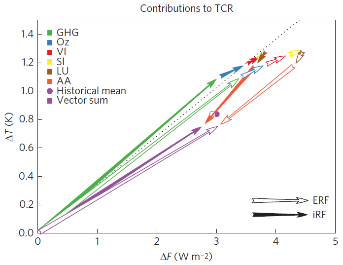
Figure 3: Reproduction of Figure 1c of Marvel et al.
As Figure 4 shows, the difference between Historical iRF and the sum of the six separate forcings closely matches, within 0.02 W/m2 in every year, SnowAlbedo_BC iRF (understood to be included in the Historical simulations) minus LU iRF. So, the difference might conceivably be due to LU iRF being missing from the Historical iRF values. If so, that would depress the efficacy estimates for Historical iRF.
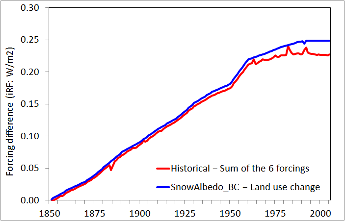
Figure 4: Differences hinting that LU iRF might be omitted from Historical forcing
Efficacy and sensitivity estimates based on iRF
Marvel et al.’s findings using iRF are a) largely irrelevant; and b) use an inappropriate estimation method. They may also use the wrong value for F2xCO2. The iRF data used is available here.
The findings using iRF are largely irrelevant because iRF is little used in observational studies, which generally use ERF and/or RF values.[12] It is therefore of little significance what efficacy, TCR and ECS estimates based on iRF values are. Marvel et al. seem to think that the IPCC AR5 RF values are iRFs, supporting their assertion that there is some ambiguity in the IPCC AR5 forcing definitions by writing: ‘For example, the best-estimate 1750–2011 iRF and ERF values given by the IPCC are identical, except for aerosols’. However, it is clear that the IPCC used RF, not iRF, values: there is no ambiguity on that point.[13] Hansen 2005 found that iRF was 56% higher than RF for ozone, 10% higher for CO2, and 5% higher for GHG and aerosols. Moreover, it is well known that, where they differ, ERF is a more appropriate measure than RF of the effect of forcings on GMST.[14] In particular, use of RF (or, a fortiori, iRF) for indirect aerosol forcing [giving RFaci] is inappropriate.[15] All three observational studies examined in Marvel et al. used ERF as a measure of aerosol forcing. Otto et al. and Lewis and Curry used ERF for non-aerosol forcings as well. None of the studies appear to have used iRF for any forcing.
The regression-with-intercept method used by Marvel et al. to estimate iRF efficacies and sensitivities is inappropriate since, although in all the simulations ΔT, ΔF and ΔQ each started at zero in 1850, in several cases the best-fit lines do not pass through or near the origin, implying that a zero forcing causes a material GMST change. That is unphysical. When either the ratio of changes since preindustrial in GMST and iRF are used instead of regression, as for ERF, or the regression best-fit lines are required to pass through the origin, substantially different iRF efficacy estimates are obtained for the forcings for land-use change, ozone, solar and volcanoes.[16]
The measure of F2xCO2 used by Marvel et al. for iRF, stated to be the model iRF value for CO2 doubling, appears instead to be the RF value in the GISS-E2-R model. Marvel et al. cites Hansen 2005 in support, but that gives values for the earlier GISS ModelE. Moreover, Hansen 2005 shows that in that model the iRF value was 10% higher, at 4.52 W/m2, than the RF value of 4.12 W/m2. The RF for doubled CO2 in the GISS E2 models is 4.1 W/m2;[17] I cannot find a published iRF value. If F2xCO2 is 10% higher in iRF than in RF terms in GISS ModelE2, as it was in GISS ModelE, then all Marvel et al.’s iRF efficacy, TCR and ECS estimates should be 10% higher.
In passing, I note that in Marvel et al.’s Figure 1 the iRF for volcanoes appears to have been shifted by +0.29 W/m2 relative to the data. No mention of this adjustment is made; the reason for it is unknown. It is unclear if it affects other results in Marvel et al.
Efficacy and sensitivity estimates based on ERF
All the ERF efficacy, TCR and ECS estimates depend on the ERF value for F2xCO2 in GISS-E2-R. Marvel et al. do not state this value and I cannot find a published value. However, giving a single set of TCR and ECS isolines for iRF and ERF in their Figure 1 implies that the same F2xCO2 value is used for both. I have therefore assumed that F2xCO2 for ERF in Marvel et al. is the same as it is for iRF, at 4.1 W/m2. However, it is arguable that the correct value is more probably ~4.5 W/m2.[18] If that is the case, all the ERF efficacy, TCR and ECS estimates should be 10% higher.
Tables 1 and 2 reproduce respectively the mean transient and equilibrium ERF efficacies stated in Table 1 of the Marvel et al. Supplementary Information (SI), along with the values I calculate from their 1996–2005 GMST data, averaged ERF data for 2000 and ocean heat uptake data (taking the trend over 1996–2005), and alternatively by accurately digitising ERF ΔF and ΔF−ΔQ values in Marvel et al. Figure 1.[19] I also show the effect of revising the ERF F2xCO2 value from 4.1 to 4.5 W/m2. For transient ERF efficacies, the relevant values from Hansen 2005 are shown for comparison. In the final row, iRF efficacies are shown to highlight where differences between ERF and iRF measures arise; a zero-intercept has been imposed when deriving the regression slopes, but no change made to Marvel et al.’s iRF F2xCO2 value.
Table 1 Transient efficacies per Marvel et al and other sources
| Forcing agent/ Source of efficacy estimates |
Aerosol AA |
Greenhouse gases GHG | Land-use change LU | Ozone Oz |
Solar SI |
Volcanoes VI |
Historical |
| Fig.1a ΔF | 0.97 | 0.95 | 2.23 | 0.62 | 0.42 | 0.53 | 0.84 |
| SI Table 1 | 0.83 | Not given | 1.81 | 0.53 | 0.35 | 0.45 | 0.71 |
| Data: unadjusted | 0.97 | 0.95 | 2.61 | 0.69 | 0.37 | 0.58 | 0.87 |
| Data: ERF F2xCO2 revised | 1.06 | 1.04 | 2.86 | 0.76 | 0.41 | 0.64 | 0.95 |
| Per Hansen 2005: Es | 0.99 | 1.02 | 1.03 | 0.90 | 0.95 | 0.88 | 0.99 |
| iRF: unadjusted data,zero-intercept slope | 1.40 | 1.04 | 1.03 | 0.70 | 1.82 | 0.31 | 0.92 |
For equilibrium efficacies, I show estimates both from the raw data (save for iRF), and with the ocean heat uptake ΔQ divided by 0.86 to estimate the full TOA imbalance ΔN and the GISS-E2-R equilibrium climate sensitivity of 2.3°C replaced by its effective climate sensitivity, taken as 2.0°C. Both these adjustments are necessary in order to estimate the efficacies fairly.
Table 2 Equilibrium efficacies per Marvel et al and other sources
| Forcing agent/ Source of efficacy estimates |
Aerosol AA |
Greenhouse gases GHG | Land-use change LU | Ozone Oz |
Solar SI |
Volcanoes VI |
Historical |
| Fig.1b ΔF-ΔQ | 0.93 | 0.83 | 1.11 | 0.56 | 0.25 | 0.48 | 0.71 |
| SI Table 1 | 0.93 | Not given | 0.11 | 0.56 | 0.26 | 0.47 | 0.71 |
| Data: unadjusted | 0.91 | 0.83 | 1.32 | 0.63 | 0.23 | 0.57 | 0.75 |
| Data: ΔQ/0.86; EffCS 2.0° | 1.14 | 1.02 | 1.48 | 0.80 | 0.27 | 0.73 | 0.92 |
| Data: F2xCO2 also revised | 1.25 | 1.12 | 1.62 | 0.87 | 0.30 | 0.80 | 1.01 |
| iRF: ΔQ/0.86; EffCS 2.0°, zero-intercept slope | 2.43 | 1.20 | 0.80 | 0.68 | 1.30 | 0.15 | 0.99 |
None of the transient efficacies given in Table 1 of the Marvel et al. SI agree to those I calculate from the data: most are 15–30% lower. Nor do any of the equilibrium efficacies agree, but the sign of the difference varies.
There are also multiple discrepancies between the ERF-based ECS estimates stated in Marvel et al. Figure 1 and those I calculate from the data, and in the ratios of efficacy to TCR and ECS estimates (which are independent of the F2xCO2 value). See Appendix B for details.
Single forcing efficacy estimates that may markedly affect observational estimation of TCR and ECS
Marvel et al. state that the GISS ModelE2 is more sensitive to CO2 alone than it is to the sum of the forcings that were important over the past century, attributing this largely to the low efficacy of ozone and volcanic forcings and the high efficacy of aerosol and LU forcing.
I have already highlighted the fact that transient efficacy for aerosol forcing is almost identical to that for CO2 when using, as in the observational studies, an ERF basis. Nor is its equilibrium ERF efficacy high.
It is well known that volcanic forcing appears to have an efficacy materially below one, at least when used in simple climate models: see the discussion in Lewis and Curry 2014.[20] But volcanic forcing barely changed between the base and final periods used in the observational studies critiqued by Marvel et al., so its efficacy is almost irrelevant to assessing them. However, in GISS-E2-R the strongly positive volcanic ERF in 1996–2005 (45 times its iRF) means that its low ERF efficacy estimate does depress efficacy and sensitivity estimates from the sum-of-six-forcings data.
Ozone forcing estimated efficacy depends on how its forcing is measured. Ozone efficacy is greater than one if the GISS-E2 ozone forcing values in Shindell et al. (2013)[21] are used instead of Marvel et al.’s.
It appears that the very high (although not statistically significant) best estimates for LU efficacy are affected by an outlier, possibly rogue, simulation run. As Figure 5 shows, run 1 produced a far higher GMST response from the middle of the 20th century on. One might expect this if simulated irrigation effects were included, but they should not have been. The difference from the ensemble mean is over four times as large as for any of the other 35 simulation runs.[22] The LU efficacies estimates are greatly reduced if run 1 is excluded. Moreover, AR5’s conclusion about the effects of land-use change imply a median estimate for LU efficacy of zero.[23]

Figure 5: GMST responses to land-use change (LU) single-forcing runs
Although Marvel et al. do not mention the very low efficacy of solar forcing in their simulations, this appears to have more effect on ERF efficacy for the sum of forcings over the historical period than does low volcanic efficacy. The efficacy of solar iRF in four non-GISS CMIP5 models has been found to be much higher than in Marvel et al.’s simulations, varying between 0.72 and 0.85.[24]
Efficacy estimates from the Historical simulation
This is the most relevant case for comparison with observational estimates, as the effect of individual forcings cannot be observed in the latter. Comparisons based on iRF data are not very relevant since observational studies do not normally use iRF. The ERF data is in principle relevant, but some of the GISS-E2-R values are difficult to believe. The GHG ERF forcing change from 1850 to 2000 is 47% higher than the corresponding change per the best estimate in AR5.[25] After allowing for F2xCO2 being 4.1 W/m2 for ERF in GISS-E2-R rather than 3.71 W/m2 in AR5, 1850–2000 GHG ERF forcing is 33% higher relative to F2xCO2 in GISS-E2-R than per AR5, despite CO2 forcing making up more than half of GHG forcing (per AR5).
This extraordinarily large difference suggests both that F2xCO2 using ERF is well above 4.1 W/m2 in GISS-E2-R, and that in that model non-CO2 GHGs produce a far higher ERF relative to CO2 than per AR5 estimates. Using a regression-based ERF F2xCO2 of 4.5 W/m2,19 TCR estimated using the Historical simulations ERF data is 1.33°C, only 5% below GISS-E2-R’s TCR of 1.4°C. And with ΔQ divided by 0.86 to better approximate ΔN, the ECS estimate is 2.02°C, in line with GISS-E2-R’s effective climate sensitivity of 1.9–2.0°C. These comparisons shows the efficacy of Historical ERF to be very close to one. Interestingly, the same is true when Historical iRF is used, provided that the iRF F2xCO2 that Hansen 2005 found for ModelE, of 4.52 W/m2, is used. In the latter case, it becomes very clear that the outlier is the WMGHG response, which has an inexplicably high efficacy. When zero-intercept regressions are used for estimation, the transient efficacy of Historical iRF is then 1.02, and the equilibrium efficacy is also 1.02 (1.09 with ΔQ divided by 0.86), based on an effective climate sensitivity of 2.0°C for the model.
Marvel et al.’s critique of observational TCR and ECS estimates from particular studies
Marvel et al. calculate TCR and ECS estimates using forcing values from Shindell 2014, Otto et al. 2013 and Lewis and Curry 2014, both with and without adjusting the efficacies of each constituent individual forcing estimate used by each. This is a pointless exercise for iRF efficacies, since none of the studies use iRF values. And it is misleading for ERF, given that several of the single forcing efficacy estimates seem very questionable. Moreover, many of the calculated TCR and ECS best estimates (medians) in their SI Table 3 do not agree to the data from their SI Tables 1 and 2.[26]
It is also the case that even had Marvel et al.’s efficacy estimates and calculations been valid, they would have had no material implications for the Otto et al 2013 TCR and ECR estimates. That is because the underlying forcing estimates used in that study already reflect efficacies, contrary to what Marvel et al. imply.
Estimates based on recent observations can only be of effective, not equilibrium, climate sensitivity, since the climate system has not reached equilibrium. It is unknown whether the two values differ to any extent in the real world. They do so in many coupled GCMs; in GISS-E2-R the effective climate sensitivity relevant to Historical forcing is ~85% of the equilibrium value. But this has nothing whatsoever to do with forcing efficacies.
Conclusions
I have highlighted many serious problems with the Marvel et al. study. Because of them, its results would be of little or no relevance to observational estimation of TCR and ECS even if the real climate system responded to forcings similarly to GISS-E2-R. Using better justified estimation methods, and the GISS-E2-R effective rather than equilibrium climate sensitivity, the Historical iRF and ERF data are both found to produce efficacies within ~10% of unity, both using Marvel et al.’s estimates of the forcing from a doubling of CO2 and with them adjusted up. Marvel et al.’s claim to have shown that TCR and ECS estimated from recent observations will be biased low is wrong. Their study lacks credibility.
Appendix A: Further information about Hansen 2005 and other efficacy-related studies
Figure A1, which reproduces Figure 25(b) of Hansen 2005, summarizes its findings for Fs. The unmarked purple range with a best estimate (open circle) of 0.9 is for ozone. When aerosol indirect effects on cloud cover were included, tropospheric (anthropogenic) aerosol efficacy reduced from 1.14 to 0.99. These efficacy estimates take into account that some forcings (e.g. aerosols, ozone and land-use change) are spatially inhomogeneous. The efficacies relate to the response 100 years after a forcing was applied. This is a longer timescale than for TCR, where the weighted mean time from forcing being imposed to measuring the response is 35 years, but it is much too short to approximate the equilibrium response.
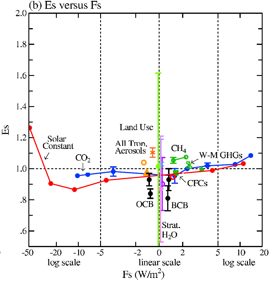
Figure A1. Reproduction of Fig. 25(b) Hansen et al (2005): Forcing efficacy relative to Fs (~ERF)
Hansen 2005 also estimated the efficacy for the sum of all the simulated transient responses to individual historical forcing changes, and for the transient response to all these forcings being applied at once. Using Fs, both efficacies were almost exactly one. This suggests that the transient responses to differing types of forcing are very comparable when forcing is taken as Fs. Hansen 2005 concluded that, at least for climate forcing agents over the historical period, Fs was a good measure of the effective forcing (the product of a forcing, however defined, and the efficacy taken relative thereto), notwithstanding that some forcings had different spatial distributions from others. However, the effect of soot (black carbon) deposited on snow and ice (SnowAlbedo_BC) was poorly constrained.
Another 2005 study,[27] which used a different model, also found that all efficacies were largely independent of the type of forcing, provided its measure accounted for tropospheric as well as stratospheric adjustment. Although the Hansen 2005 results were based on the behaviour of a single GCM, they were generally supported in AR5, which concluded that ERF is a better measure than RF of the eventual GMST response, especially for aerosols, although in most cases the difference was small. SnowAlbedo_BC forcing was, exceptionally, estimated to cause a two to four times larger GMST change relative to its RF than does CO2.
Subsequent to AR5, another NASA GISS scientist, Drew Shindell, published a study (Shindell 2014)[28] claiming that the transient response to spatially inhomogeneous forcings was significantly greater than that to GHGs, with the consequence that estimates of TCR based on comparing GMST and total forcing changes since circa 1850 were biased down. The dominant spatially inhomogeneous forcing is that from aerosols, but ozone and, to a minor extent, land-use change also contribute. Shindell’s study was based on comparing historical simulations with all forcings, GHG-only and natural-only forcings included. This is a less clean approach than using single-forcing simulations. It requires making various difficult-to-assess assumptions and adjustments, and magnifies the noise from model internal variability.
I find Shindell’s results difficult to reconcile with the observed evolution of hemispherical and tropical temperatures relative to GMST over the historical period. Moreover, they are contradicted not only by Hansen’s 2005 study, but also (in respect of aerosols) by the only other relevant published single forcing simulation based study [29] that I know of apart from Marvel et al. I am also aware of as yet unpublished work using another, state-of-the-art, GCM that likewise shows no evidence of a greater transient response to aerosol forcing than to CO2.
For completeness, I will add that following Shindell’s study, Kummer and Dessler published a paper[30] applying Shindell’s finding, that the efficacy of aerosol and ozone forcing was about 1.5, to the estimation of ECS, thereby obtaining a central value for ECS of over 3°C. Clearly, if Shindell’s findings are invalid, so are Kummer and Dessler’s.
Appendix B: Discussion of discrepancies in Marvel et al.’s ERF based TCR and ECS estimates
Marvel et al. state, in their Figure 1 legends, TCR and ECS estimates for GISS-E2-R implied for ERF basis forcings by the ΔT and ΔF−ΔQ values. The ECS values should be compared with the model’s effective climate sensitivity of 1.9–2.0°C. A comparison of the stated values with those calculated from the ΔT, ΔF and ΔQ data and from digitised values for ΔF−ΔQ is given in Table 3. Marvel et al.’s values almost all disagree, by varying ratios, with either of those I calculate. The last row of each section of Table 3 shows what the TCR and ECS estimates calculated from data revised as indicated would be.
Table 3: Marvel et al.’s ERF-based TCR and ECS estimates and recalculated equivalents
| Forcing agent/ Type & source of sensitivity | Aerosol AA |
Greenhouse gases GHG | Land-use change LU | Ozone Oz |
Solar SI |
Volcanoes VI |
Historical |
| TCR: per Fig.1a ΔF | 1.36 | 1.32 | 3.13 | 0.88 | 0.58 | 0.75 | 1.17 |
| TCR: stated in Fig.1a | 1.3 | 1.2 | 2.8 | 0.8 | 0.5 | 0.7 | 1.1 |
| TCR: on unadjusted data | 1.35 | 1.33 | 3.65 | 0.97 | 0.52 | 0.82 | 1.21 |
| With F2xCO2 revised | 1.49 | 1.46 | 4.00 | 1.06 | 0.57 | 0.90 | 1.33 |
| ECS: per Fig.1b ΔF−ΔQ | 2.14 | 1.90 | 2.54 | 1.28 | 0.58 | 1.12 | 1.64 |
| ECS: stated in Fig.1b | 2.0 | 1.7 | 2.4 | 1.2 | 0.5 | 1.0 | 1.5 |
| ECS: on unadjusted data | 2.08 | 1.90 | 3.04 | 1.46 | 0.54 | 1.32 | 1.72 |
| ΔQ/0.86; F2xCO2 revised | 2.50 | 2.25 | 3.25 | 1.75 | 0.60 | 1.61 | 2.02 |
Whatever the ERF F2xCO2 value used in Marvel et al. is, for every forcing agent the ratio of the ERF-based TCR stated in its Figure 1a to the ERF transient efficacy given in its SI Table 1 should equal the GISS-E2-R TCR of 1.4°C, and the ratio of the ERF ECS stated in their Figure 1b to the ERF equilibrium efficacy given in their SI Table 1 should equal the GISS-E2-R ECS of 2.3°C. However, save for solar forcing, the ratios calculated from the data imply a model TCR of 1.51–1.57°C, ~10% higher than its 1.4°C TCR. For ECS, omitting the obviously incorrect LU efficacy, all the ratios imply model ECS values in the range 2.11–2.15°C, nearly 10% lower than its 2.3°C ECS, again save for solar, which is further adrift.
[1] Kate Marvel, Gavin A. Schmidt, Ron L. Miller and Larissa S. Nazarenko, et al.: Implications for climate sensitivity from the response to individual forcings. Nature Climate Change DOI: 10.1038/NCLIMATE2888. The paper is pay-walled, but the Supplementary Information (SI) is not.
[2] The Historical simulations have an average temperature anomaly of 0.84°C for 1996–2005 relative to 1850, whereas HadCRUT4v4 shows an increase of 0.73°C from 1850–1859 to 1996–2005, and Figure 7 of Miller et al. 2014 shows consistently greater warming for GISS-E2-R than per GISTEMP since 2000. The same simulations show average ocean heat uptake of 0.84 W/m2 over 1996–2005 (mean slope estimate), compared to 0.40 W/m2 using AR5 Box 3.1, Figure 1 data, or 0.67 W/m2 using NOAA (Levitus et al. 2012) data.
[3] Hansen J et al (2005) Efficacy of climate forcings. J Geophys Res, 110: D18104, doi:101029/2005JD005776
[4] Chapter 8 of AR5 is available here.
[5] See Section 10.8.1 in Chapter 10 of AR5 for a discussion of the use of these equations in estimating TCR and ECS.
[6] Miller, R. L. et al. CMIP5 historical simulations (1850_2012) with GISS ModelE2. J. Adv. Model. Earth Syst. 6, 441_477 (2014).
[7] Or with climate state, but feedbacks vary little with climate state, within limits, in most GCMs.
[8] I estimate GISS-E2-R’s effective climate sensitivity applicable to the historical period as 1.9°C and its ERF F2xCO2 as 4.5 Wm−2, implying a climate feedback parameter of 2.37 Wm−2 K−1, based on a standard Gregory plot regression of (ΔF − ΔN) on ΔT for 35 years following an abrupt quadrupling of CO2 concentration. The efficacy-weighted mean period from the imposition of incremental forcing to the end of the historical period is of this order. I also estimate the model’s effective climate sensitivity, as 2.0°C, from regressing the same variables over the first 100 years of its 1% p.a. CO2 increase simulation; this estimate is little affected by F2xCO2 value.
[9] Miller et al. 2014 noted a 15% increase in GHG forcing in GISS ModelE2 compared to the CMIP3 version ModelE, despite their forcing (RF) for a doubling of CO2 being nearly identical, but were unable to identify the cause.
[10] The 0.86 divisor comes from the coefficient on the integral of TOA imbalance anomaly ΔN when regressing the ocean heat content (OHC) anomaly against both that integral and time, thus isolating any fixed offset between ΔQ and ΔN that may exist.
[11] The 1996-2005 ΔT for the sum of the six single-forcing cases is 0.76°C, compared to 0.84°C for Historical (all forcings). For iRF, the corresponding ΔF values from the archived data are 2.53 W/m2 and 2.75 W/m2. However, the values plotted are 2.74 W/m2 and 3.05 W/m2 respectively. For ERF, the sum-of single forcings and the Historical forcing ΔF values from the data are respectively 2.99 W/m2 and 2.84 W/m2, but the values plotted in Figure 1c are 3.03 W/m2 and 2.93 W/m2.
[12] Otto et al. used regression-based estimates of ERF in multiple CMIP5 models. Lewis and Curry used estimates from Table AII.1.2 of AR5, which are stated to be ERFs but in most cases (aerosol forcing being the most notable exception) assessed to be the same as their RFs.
[13] The AR5 Glossary (Annex III) states: ”The traditional radiative forcing is computed with all tropospheric properties held fixed at their unperturbed values, and after allowing for stratospheric temperatures, if perturbed, to readjust to radiative-dynamical equilibrium. Radiative forcing is called instantaneous if no change in stratospheric temperature is accounted for.” And early in Chapter 8 it says: ”RF is hereafter taken to mean the stratospherically adjusted RF.”
[14] However, Hansen 2005 found that only in the cases of aerosol and BCsnow forcing was there a major difference between RF and ERF. AR5, after surveying a wider range of evidence, reached similar conclusions, and accordingly in other cases estimated ERF to be the same as RF, with an implied efficacy estimate of one, but gave wider ranges for ERF to allow for uncertainty in the relationship between ERF and RF.
[15] AR5 states (Section 7.5.1 of Chapter 7): ”it is inherently difficult to separate RFaci from subsequent rapid cloud adjustments either in observations or model calculations… For this reason estimates of RFaci are of limited interest and are not assessed in this report.”
[16] Transient efficacy estimates using iRF based respectively on unconstrained decadal regression from 1906–2015 to 1996–2005 (as in Marvel et al.), changes from 1850 to 1996–2005, and zero-intercept regression are: LU 3.89, 1.64, 1.03; Oz 0.60, 0.57, 0.70; SI 1.53, 1.68, 1.82; and VI 0.56, 26.45, 0.31. In principle, using changes is preferable to zero-intercept regression for transient estimation because of the ‘cold start’ issue, but its superior noise suppression leads to more consistent estimation from zero-intercept regression when forcing is small.
[17] Schmidt, G. A., et al. (2014): Configuration and assessment of the GISS ModelE2 contributions to the CMIP5 archive, J. Adv. Model. Earth Syst., 6, 141–184, doi:10.1002/2013MS000265.
[18] The GHG forcing in 1996–2005 is 10% higher in ERF than in iRF terms. GHG forcing in 1996–2005 was dominated by CO2, and Hansen 2005 found GHG had an efficacy of very close to one both in terms of Fs, which is very similar to ERF, and using iRF (1.02 and 1.04 respectively). That suggests scaling the actual F2xCO2 iRF of 4.1 W/m2 by the ratio of Marvel et al.’s iRF and ERF values for GHG forcing, which implies a 10% higher F2xCO2 ERF, of 4.52 W/m2. That value is also in line with F2xCO2 of 4.53 W/m2 estimated from a Gregory-plot regression over the 35 years following an abrupt quadrupling of CO2.
[19] There were no material differences between the digitised and data values for ΔT, so I used only the data values, which were more precise. Note that Marvel et al. do not specify whether, for ERF efficacy estimates, ensemble means are taken before or after calculating quotients. As only a single forcing value is given, and ensmble means were taken before regressing in the iRF case, I have assumed the former, which also seems more appropriate.
[20] Lewis N, Curry JA (2014) The implications for climate sensitivity of AR5 forcing and heat uptake estimates. Clim. Dyn. DOI 10.1007/s00382-014-2342-y. Non-typeset version available here.
[21] Shindell, D. T., et al., 2013: Interactive ozone and methane chemistry in GISS-E2 historical and future climate simulations. Atmos. Chem. Phys., 13, 2653–2689. This study found that iRF ozone forcing from 1850 to 2000.was 0.28 W/m2 when the climate state was allowed to evolve in line with the Historical simulation and 0.22 W/m2 when a fixed present-day climate was used, and ERF was calculated as 0.22 W/m2. These values are substantially below those used in Marvel et al. of 0.45 W/m2 iRF and 0.38 W/m2 ERF. Substituting Shindell et al.’s values for Marvel et al.’s would raise the ozone iRF and ERF transient efficacies values to respectively 0.92 and 1.18.
[22] If one excludes LU run 1, no individual run for any forcing (including Historical) produces a 1950-2005 mean GMST response that differs by more than 0.031°C from the ensemble mean response for that forcing. But for LU run 1 the difference is -0.134°C (and would be -0.168°C were run 1 excluded from the ensemble mean).
[23] Chapter 8 of AR5, referring to a seven model study, states that ”There is no agreement on the sign of the temperature change induced by anthropogenic land-use change” and concludes that a net cooling of the surface – accounting for processes that are not limited to the albedo—is about as likely as not”.
[24] Schmidt H et al. (2012) Solar irradiance reduction to counteract radiative forcing from a quadrupling of CO2: climate responses simulated by four earth system models Earth Syst. Dynam., 3, 63–78
[25] The GISS-E2-R increase in GHG ERF is 3.39 W/m2. The 1850-2000 increase in GHG RF and ERF per AR5 Table AII.1.2 is 2.25 W/m2, but I use the higher 1842–2000 increase of 2.30 W/m2 since the 1850 CO2 concentration in GISS ModelE2 was first reached in ~1842, according to the AR5 data.
[26] I calculate TCR and ECS values as shown in the below table, from the efficacies stated in Marvel et al.’s SI Table 1 (digitising from their Figure 1 for GHG). [E=1 means assuming all efficacies are one.]
| Median estimates | Shindell 2014 | Lewis and Curry 2014 | Otto et al 2013 | |||||||
| E=1 | iRF | ERF | E=1 | iRF | ERF | E=1 | iRF | ERF | ||
| TCR | ||||||||||
| As stated in SI Table 3 | 1.4 | 2.0 | 1.9 | 1.3 | 1.6 | 1.7 | 1.3 | 1.8 | 1.8 | |
| From SI Table 1 (GHG from Fig.1) | 1.98 | 1.58 | 1.92 | 1.60 | 1.92 | 1.69 | ||||
| ECS | ||||||||||
| As stated in SI Table 3 | 2.1 | 4.0 | 3.6 | 1.5 | 2.0 | 2.3 | 2.0 | 2.9 | 3.4 | |
| From SI Table 1 (GHG from Fig.1) | 3.88 | 3.48 | 2.77 | 2.73 | 3.90 | 3.78 | ||||
[27] Sokolov, A P (2005): Does model sensitivity to changes in CO2 provide a measure of sensitivity to other forcings? J Climate, 19, 3294-3305
[28] Shindell, DT (2014) Inhomogeneous forcing and transient climate sensitivity. Nature Clim Chg: DOI: 10.1038/NCLIMATE2136
[29] Ocko IB, V Ramaswamy and Y Ming (2014) Contrasting climate responses to the scattering and absorbing features of anthropogenic aerosol forcings. J. Climate, 27, 5329–5345.
[30] Kummer J. R. and A. E. Dessler (2014): The impact of forcing efficacy on the equilibrium climate sensitivity. GRL, 10.1002/2014GL060046
Update: Data and calculations are available here, in Excel form
Leave A Comment