Originally a guest post on Jan 21, 2016 – 12:08 PM at Climate Audit
Introduction
In a recent article I discussed the December 2015 Marvel et al.[1] paper, which contends that estimates of the transient climate response (TCR) and equilibrium climate sensitivity (ECS) derived from recent observations of changes in global mean surface temperature (GMST) are biased low. Marvel et al. reached this conclusion from analysing the response of the GISS-E2-R climate model in simulations over the historical period (1850–2005) when driven by six individual forcings, and also by all forcings together, the latter referred to as the ‘Historical’ simulation. The six individual forcings analysed were well-mixed greenhouse gases (GHG), anthropogenic aerosols, ozone, land use change, solar variations and volcanoes. Ensembles of five simulation runs were carried out for each constituent individual forcing, and of six runs for all forcings together. Marvel et al.’s estimates were based on averaging over the relevant simulation runs; taking ensemble averages reduces the impact of random variability.
In this article I will give a update on the status of two points I tentatively raised in my original article.
Land use change (LU) forcing
I commented in my original article that LU run 1 showed a much more negative GMST response than any of runs 2 to 5, from the middle of the 20th century on (see Figure 5 in the original article). I conjectured that run 1 might be a rogue. Excluding it reduces the transient efficacy for iRF from 3.89 to 2.48, and that for ERF from 2.61 to 1.75, with both iRF and ERF equilibrium efficacies reduced to around one.
I have now downloaded and processed CMIP5 data for the GISS-E2-R single forcing runs, so I can show the spatial effects of LU forcing on simulated surface temperatures.
First, I show (Figure 1) the spatial distribution of Land use forcing applied in the model simulations during 2000. Its global mean value is −0.19 W/m2, but the forcing is very concentrated in particular regions. The forcing increases gradually from zero in 1850, flattening out after ~1960.
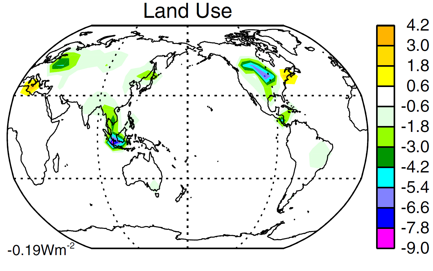 Figure 1. Reproduction of Figure 4c from Miller et al 2014:[2] LU forcing in 2000 (vs 1850)
Figure 2 shows the changes simulated by GISS-E2-R in response to LU forcing for each of simulation runs 2 to 5. They compare mean temperatures over 1976–2000 with those over 1850–75. Note that longitudes in these world maps are centred on Greenwich rather than the Pacific.
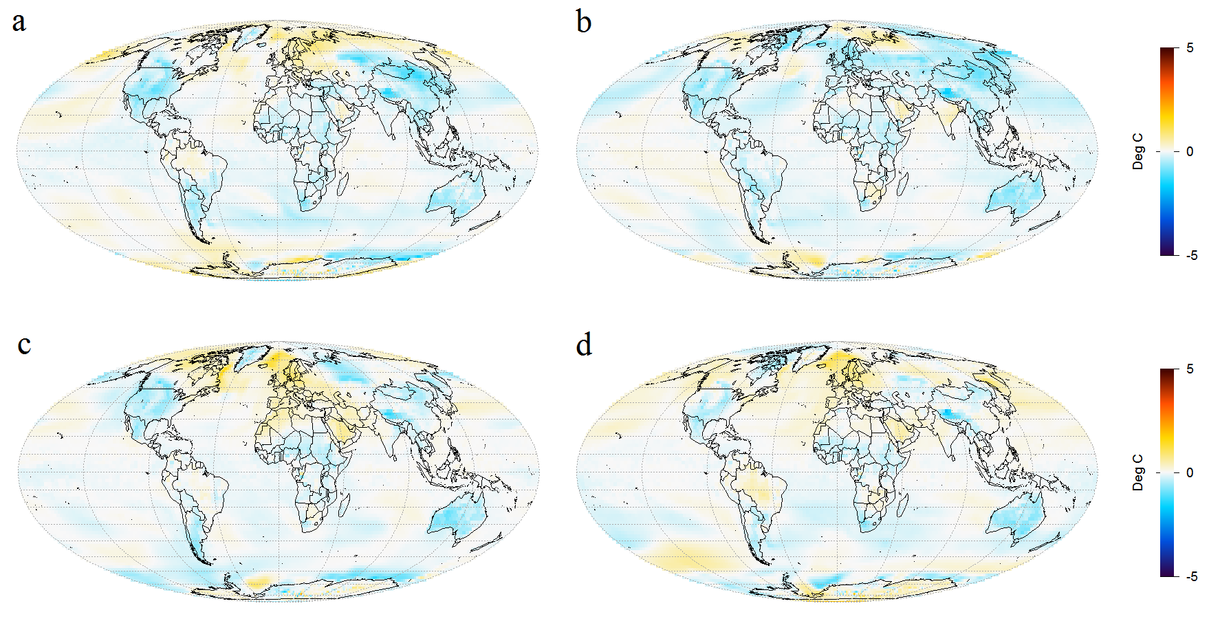
Figure 2. Simulated surface temperature change (1850–75 to 1976–2000 mean) driven by land use change forcing only: maps a to d show results from runs 2 to 5 respectively.
As the forcing and resulting temperature changes are small, internal variability has a significant effect on simulated changes even when comparing 25 year means, with changes varying in sign over some land areas and most of the ocean. Figure 3, which shows the average of all the plots in Figure 2, confirms that temperature changes are small everywhere. Globally averaged, there is a cooling of 0.04°C. Note that the temperature scale has been halved in Figure 3; taking the average of four runs halves variability.
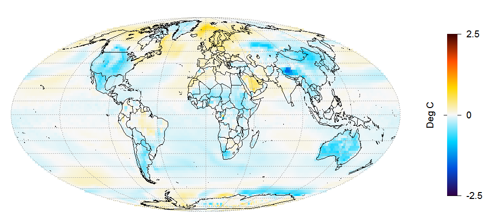 Figure 3. Average of temperature changes for runs 2 to 5, as plotted in Figure 2.
Figure 3 also shows that although LU forcing is very spatially inhomogeneous, it affects temperatures throughout the globe. The generally greater cooling in land masses than over the ocean is mainly due to temperatures over land generally being more sensitive to global forcing, not to LU forcing being located in land masses. Broadly, in GCMs a local forcing has a global effect, with local temperature changes being determined more by local climate sensitivity (the reciprocal of climate feedback strength) than by local forcing. Forcing from black carbon deposited on snow is a partial exception to this rule; it is concentrated at high latitudes, from which heat is less readily transported elsewhere. The way in which GCMs spread globally the effects of local forcings accords quite well with a physical understanding of how the climate system works. And it explains why, when a measure of forcing (ERF) that allows the troposphere to adjust to its presence is used, most forcings are thought to have an efficacy close to one despite some of them being quite spatially inhomogeneous.
The temperature changes simulated in run 1, shown in Figure 4, are very different.
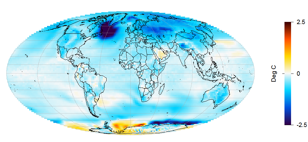
Figure 4. LU run 1 surface temperature change from 1850–75 to 1976–2000 mean.
A very cold anomaly has developed in the ocean south of Greenland. In most of the dark blue patch, the temperature has dropped by over 3°C, and by over 5°C in the centre of this area. Additional cooling to that shown in runs 2–5 has developed almost everywhere, apart from off Antarctica, where some areas have warmed strongly and others cooled strongly. This all seems to point to some major change in the ocean overturning circulation having occurred in this run, resulting in the cold ocean anomaly south of Greenland and substantial surface cooling in most areas.
I drew this finding to the attention of Ron Miller of GISS, one of the Marvel et al. authors, last week, asking whether he had any explanation and enquiring whether the simulation might be rerun, as GISS had done when another single forcing run had, for unknown reasons, an unreproducable excursion in the middle of the run. I have now heard back from Ron Miller to the effect that, although LU run 1 indicates greater cooling, he doesn’t regard the run as pathological and can’t see any reason to treat it differently, and that they don’t have any current plans to rerun this simulation.
Whatever the exact cause of the massive oceanic cold anomaly developing in the GISS model during run 1 , I find it very difficult to see that is has anything to do with land use change forcing. And whether or not internal variability in the real climate system might be able to cause similar effects, it seems clear that no massive ocean temperature anomaly did in fact develop during the historical period. Therefore, any theoretical possibility of changes like those in LU run 1 occurring in the real world seems irrelevant when estimating the effects of land use change on deriving TCR and ECS values from recorded warming over the historical period.
Possible omission of land use change forcing from Historical forcing data values
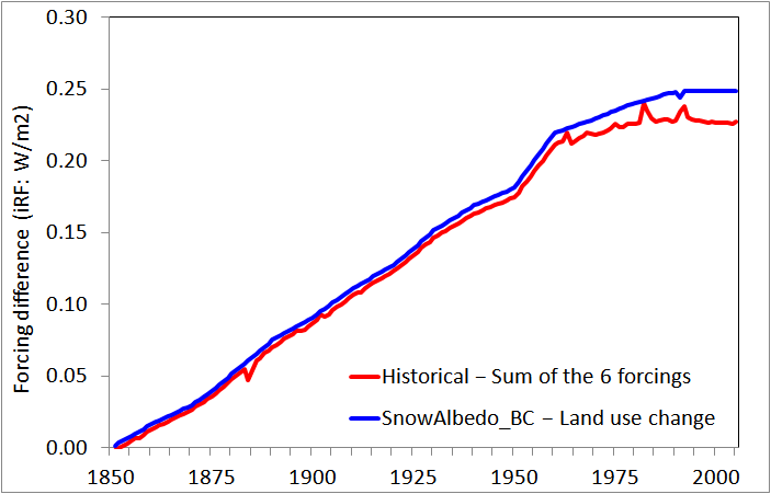
I noted in my original article that the differences between the GISS Historical forcing data (iRF time series) and the sum of those for the constituent individual forcings suggested that, unlikely as it might seem, the negative contribution from land use change forcing might have been omitted from the Historical forcing values. My Figure 4 showed that when LU forcing was deducted, the excess of Historical forcing over the sum of the six individual forcings analysed by Marvel et al. almost exactly matched forcing from black carbon deposited on snow and ice (Snow Albedo BC), a minor forcing included in the Historical simulations in addition to the six forcing analysed in Marvel et al.
Omission of LU forcing values would have increased Historical forcing values, thereby (assuming that LU forcing had nevertheless actually been applied in the Historical simulations) causing a downwards bias of ~5% or so in estimates of efficacy and TCR/ECS derived from the Historical simulations. By contrast, the inclusion in the Historical simulation forcing values of Snow Albedo BC forcing does not cause a bias since its effects on GMST and heat uptake are reflected in the Historical simulations; likewise for the trivially small (<0.0025 W/m2) orbital forcing. However, it is difficult to see how the Historical simulation could have included LU forcing without the value of LU forcing being included in the Historical forcing values. That is because, as I understand it from reading Miller et al. 2014, the Historical forcing values were derived from the Historical simulation radiation data, not by adding up individual forcing values derived from the constituent single forcing simulations.
Nevertheless, I decided to investigate this issue by multiple regression of Historical forcing against the constituent forcing series. This approach is based on the standard assumption that individual forcings are linearly additive. Although in reality any climate-state dependence of individual forcings would make this assumption inaccurate, here all the iRF values have been calculated with a fixed 1850 climate state, before perturbation by any applied forcings, so I would expect linear additivity to be a good approximation.
I used annual data over 1851–2012, being all data except for the baseline year of 1850, when all forcing values were zero. I started the regression in 1851 as there appeared to be a ~0.004 W/m2 jump in Historical forcing relative to the sum of individual forcings between 1850 and 1851. I therefore added 0.004 W/m2 to the Historical forcing values and then regressed with no intercept term. I started by regressing on all nine series: there are separate series for direct and indirect aerosol forcing. Table 1 shows the results.
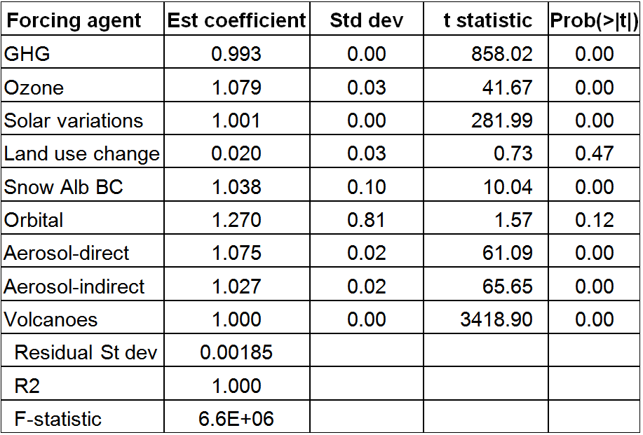 Table 1. Results from regressing all Historical forcing on all individual forcings over 1851-2012
Land use forcing has a regression coefficient negligibly different from zero, whereas all other forcings have regression coefficients close to one. This result provides further evidence that LU forcing may not be included in the Historical forcing values. The fit is extremely good: the residual standard deviation is under 0.1% of Historical forcing in 2000. However, given the similarity between most of the forcing time series – which apart from volcanoes and solar variation all increase smoothly over time – the estimation uncertainty will be greater than appears from the coefficient standard deviation values. Therefore, even though the modest excesses over one of the Aerosol-direct and Ozone coefficients are three or four times the standard deviation estimates, it is difficult to see them as being at all significant.
Regressing against so many variables, most of which are highly collinear, can give misleading results. I therefore reduced the number of variables to five by dropping the tiny Orbital forcing and aggregating some other forcings. The results (Table 2) show almost as low a residual standard deviation as before, and an even smaller coefficient on Land use change forcing. Dropping LU forcing as a regressor does not increase the residual standard deviation of 0.00195, but brings the estimated coefficients for Aerosol + Ozone and for Snow Albedo BC down to somewhat closer to one. Adding a very small amount (< 0.004 W/m2) of random noise to the annual Historical forcing values also affects those two coefficients, making them fluctuate around one without significantly affecting the remaining coefficients. If I aggregate all non-LU forcings together and just regress on that and LU forcing, the residual standard deviation goes up but the coefficient on LU remains almost zero.
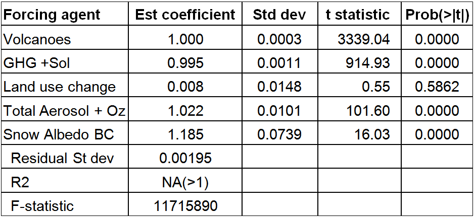 Table 2. Results from regressing all Historical forcing on five forcings over 1851-2012
The regression residuals from the Table 2 regression (Figure 5) are dominated by spikes at the time of volcanic eruptions, the origin of which is unclear.
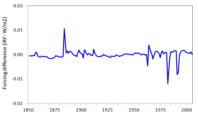 Figure 5. Residuals from regressing all Historical forcing on five forcings over 1851-2012
I am at a bit of a loss to make sense of these results. I have considered the possibility that stratospheric water vapour forcing might account for the excess of Historical forcing values over the sum of all the individual forcing values. Stratospheric water vapour forcing is not imposed or calculated separately in GISS-E2-R, but arises from the oxidation of methane.[3] It is thought to be similar to that in GISS ModelE, which was estimated as ~0.07 W/m2 in 2000 relative to 1850 – only about a third of the unexplained excess. Moreover, as the iRF estimation method involves the climate state – including water vapour and clouds – being fixed in 1850, it does not appear that stratospheric water vapour forcing would be included in Historical iRF (nor in GHG iRF).
The most logical explanation I can find for the regression results is that land use forcing was somehow inadvertently entirely omitted from the GISS-E2-R Historical simulations, not just from the archived Historical forcing values. But that would seem quite an unlikely mistake. A second possibility is that there is some flaw in my regression approach or its implementation, or that I am overlooking something obvious. Another possibility is that some interaction between forcings that detracts from linear additivity mimics subtracting Land use forcing, although what interaction might produce an appropriately shaped time profile is not obvious. Perhaps one of those explanations is more likely than that GISS slipped up. I really don’t know what the explanation is for the apparently missing Land use forcing. Hopefully GISS, who alone have all the necessary information, may be able to provide enlightenment.
Response from the authors generally
The only substantive response to date from the authors of Marvel et al. to my original article, other than regarding LU run 1, has been a comment at RealClimate by Gavin Schmidt, stating that my observation that their plotted iRF values (both for volcanoes and historical forcing) appear to be shifted by +0.29 W/m2 from the data values was misplaced, since they had used 1850–59 mean forcings as a baseline. There was no mention anywhere in Marvel et al. that this had been done. The difference is negligible except for volcanic (and hence also Historical) forcing: all other individual forcings varied very little during the 1850s from their value in 1850, the baseline year used for the data values.
The baseline used for iRF forcings is not actually relevant to my criticisms of results in Marvel et al. Since their iRF results are based on regressions over 1906–2005, with the estimated best-fit lines not constrained to pass through the zero-forcing, zero-GMST change origin, they are unaffected by the baseline used. Revising the forcing baseline alters, for volcanic and Historical forcings, the differences between Marvel’s best-fit slope and that derived from a more physically-justifiable regression basis that requires it to pass through the origin, but it does not eliminate them.
The use of a 1850–59 baseline also greatly reduces the apparent large difference between iRF and ERF volcanic forcing changes. However, that does not affect my point that the strongly positive change in low-efficacy ERF volcanic forcing to 1996–2005 depresses the TCR/ECS estimates based on Historical ERF forcing in a way that is not applicable to most observationally-based estimates. This point applies equally to the Marvel et al. iRF based estimates. The downwards bias that low volcanic forcing efficacy has on estimation of TCR and ECS from the Historical simulations would not occur if the practices used in sound observationally-based, historical period studies were followed. Such studies use analysis periods or methods that minimise the impact of volcanism, and thereby avoid bias from low volcanic efficacy.
Acknowledgements
I thank Ryan O’Donnell for the code used to produce the World projection plots.
[1] Kate Marvel, Gavin A. Schmidt, Ron L. Miller and Larissa S. Nazarenko, et al.: Implications for climate sensitivity from the response to individual forcings. Nature Climate Change DOI: 10.1038/NCLIMATE2888. The paper is pay-walled, but the Supplementary Information (SI) is not.
[2] Miller, R. L. et al. CMIP5 historical simulations (1850_2012) with GISS ModelE2. J. Adv. Model. Earth Syst. 6, 441_477 (2014). Open access.
[3] According to Miller et al. 2014, stratospheric water vapour is augmented according to the surface methane concentration, with a prescribed 2 year lag. Calculation of the forcing due to oxidation of methane is complicated, because several years elapse before the water vapour originating as surface methane circulates throughout the stratosphere.
Update 23 January 2016
I have just discovered (from Chandler et al 2013) that there was an error in the ocean model in the version of GISS-E2-R used to run the CMIP5 simulations. The single forcing simulations were part of the CMIP5 design, although it is possible that some or all of them were run after the correction was implemented.
Chandler et al write:
” We discuss two versions of the Pliocene and Preindustrial simulations because one set of simulations includes a post-CMIP5 correction to the model’s Gent-McWilliams ocean mixing scheme that has a substantial impact on the results – and offers a substantial improvement, correcting some serious problems with the GISS ModelE2-R ocean.”
explaining the problem as follows:
“the simulations described here as “GM-CORR” utilise a correction to the Gent- McWilliams parameterisation in the ocean component of the coupled climate model. In prior implementations of the mesoscale mixing parameterisation in GISS ModelE, which like many ocean models uses a unified Redi/GM scheme (Redi, 1982; Gent and McWilliams, 1990; Gent et al., 1995; Visbeck et al., 1997), a miscalculation in the isopycnal slopes led to spurious heat fluxes across the neutral surfaces, resulting in an ocean interior generally too warm, but with southern high latitudes that were too cold. A correction to resolve the problem was made for this study, and it will also be employed in all subsequent versions of ModelE2-R going forward.”
Interestingly, they also write:
“One of the most significant differences of the Pliocene GM CORR simulations, compared with those of the uncorrected model, is the characteristic of the meridional overturning in the Atlantic Ocean. In GM UNCOR the Atlantic Meridional Overturning Circulation (AMOC) collapsed and did not recover, something that was expected to be related to problems with the ocean mixing scheme. Although we hesitate to state that this is a clear improvement (little direct evidence from observations), it seems likely that the collapsed AMOC in the previous simulation was erroneous.”
It occurs to me to wonder whether this error in the GISS-E2-R ocean mixing parameterisation may account for its behaviour in Land use change run 1. It looks like something goes seriously wrong with the AMOC in the middle of the 20th century in that run, with no subsequent recovery evident. I have been unable to ascertain as yet whether that simulation was run using the uncorrected or the corrected ocean module code.
Additional reference: Chandler M A et al, 2013. Simulations of the mid-Pliocene Warm Period using two versions of the NASA/GISS ModelE2-R coupled model. Geosci Model Dev. 6, 517–531 (Open access)
Update 31 January 2016
I have now uploaded GMST and top of atmosphere radiative imbalance data from 1850 on for the GISS-E2-R runs used in Marvel et al. The data used by Marvel et al, available on the GISS website, omitted the first 50 years of simulations in the case of the GMST data, and gave ocean heat content rather than the appropriate, approximately 16% larger, TOA radiative imbalance data .
Leave A Comment