Original a guest post on July 7, 2011 at Climate Etc.
JC note: Pursuant to Nic’s post on “The IPCC’s alteration of Forster & Gregory’s model-independent climate sensitivity results,” he has sent a letter to Gabi Hegerl, who was coordinating lead author on chapter 9 of the IPCC AR4.
Dear Gabi,
I asked you yesterday whether you were aware that two of the climate sensitivity PDFs in Figure 9.20 of the IPCC AR4 WG1 report were not in fact based on a uniform prior in equilibrium climate sensitivity (ECS or S), despite it being stated in Table 9.3 that they were so based. I stated that one PDF was effectively based on a uniform prior in the climate feedback parameter (Y or λ), which rather detracted from the IPCC’s case for transforming the Forster/Gregory 06 results from that basis to a uniform prior in ESC basis.
You responded saying that you would be surprised if there was an error in the Figure as the Table and Figure had been double checked with paper authors, but if there was an error you would like to know.
The Figure 9.20 climate sensitivity PDF that is effectively based on a uniform prior in the climate feedback parameter Y is that for Gregory 02. As it happens, the arguments for that being the correct basis are very similar to the arguments applying in the case of Forster/Gregory 06. In both cases the (assumed linear) physical relationship between observables that is being estimated relates to Y (or λ), not S, and the error characteristics are similar – assumed gaussian, with errors in temperature data dominated by errors elsewhere.
Why do I say that the PDF for Gregory 02 in Figure 9.20 – which is almost the same as that in the original paper – is effectively based on a uniform prior in Y or λ, not a uniform prior in ESC as stated? Gregory 02 estimated λ from the equation Q – F = λ ΔT , where Q is imposed radiative forcing, F is heat flux into the ocean and ΔT is the change in global average surface temperature, underbars indicating the difference in means thereof between 1861–1900 and 1957–1994.
As one would expect, due to errors in Q and F being dominant and being assumed to have a gaussian distribution, the PDF for the climate feedback parameter has an almost gaussian distribution. The situation is very similar to that in Forster/Gregory 06, where it was correctly stated:
“For the uncertainty analysis we assume, like Gregory et al. (2002), that errors in the observable parameters (N, Q, and ΔTs) all have Gaussian distributions. In a Bayesian statistics framework, this is equivalent to assuming Gaussian observational errors and a uniform “prior” in each of the observables. Since the uncertainties in Q and N are much larger than in ΔTs (a factor influencing our choice of regression model; see appendix), uncertainty in Q – N is linearly related to uncertainty in Y, so our assumption is also approximately equivalent to assuming a uniform prior in Y.”
In Gregory 02, the estimate of Y is not obtained by regression in the usual sense of the word: as there are only two observations (the means for 1861–1900 and for 1957–1994) a perfect straight line fit results. But, as in Forster/Gregory 06, uncertainty in Q – F is linearly related to uncertainty in Y, and it is equally the case that the error assumptions in Gregory 02 are approximately equivalent to assuming a uniform prior in Y.
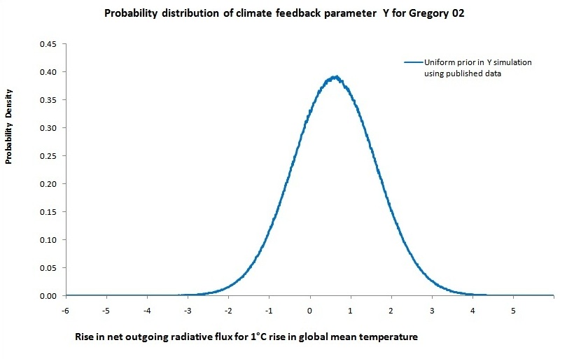
The estimated PDF for the climate feedback parameter Y was not shown in Gregory 02. Figure 1 below shows what I calculate it looks like. The PDF has been computed in the same way (apart from the reciprocal relationship) as the climate sensitivity PDF in Figure 2 in the original paper, using the same data and error distribution assumptions but with a larger number of random samples to improve accuracy.

Figure 1
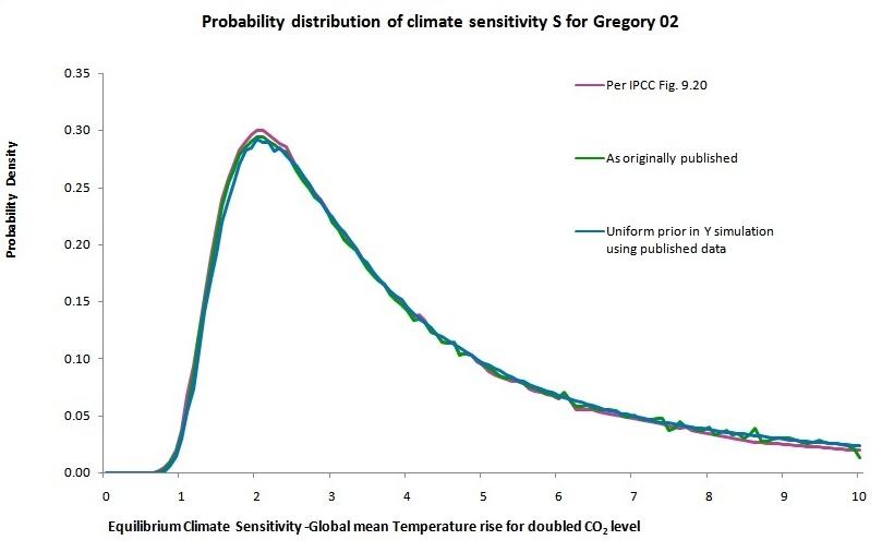
Gregory 02 in fact computed the probability distribution of the climate sensitivity directly from the random samples of the variables. The PDF from their paper (Fig. 2) is shown as the green line in Figure 2, below. The PDF from Figure 9.20 of AR4 WG1 is shown as the magenta line.
The blue line in Figure 2 shows my calculation of the PDF for climate sensitivity S, derived by a simple inversion of the PDF for Y shown in Figure 1. By simple inversion I mean that given by the standard rules of probability for converting PDFs between two parameters, being multiplication by the absolute value of the derivative of the old parameter with respect to the new one, or by 3.7/S2 in this case, and renormalization. That procedure does not involve any change to the effective prior distribution used, which remains approximately uniform in Y. My blue line is virtually identical to the green line from the Gregory 02 paper, except that as I used a larger sample size my line is less jagged.
The small differences between the three lines are due partly to digitization errors, partly to fluctuations caused by the restricted sample size used in the Gregory 02 paper, and partly to smoothing in Figure 9.20.
Figure 2
As in the actual IPCC Figure 9.20, climate sensitivity in Figure 2 has been truncated over the range 0 – 10°C. In the case of Gregory 02, doing so involves a substantial truncation of the distribution of S at the top end. In fact, there is a considerable area of the PDF for Y below Y=0, which can be ruled out by the long term stability of the Earth’s climate. That suggests to me that the Gregory 02 estimate of Q may be too low and/or its estimate of F too high. I will come back to this point later.
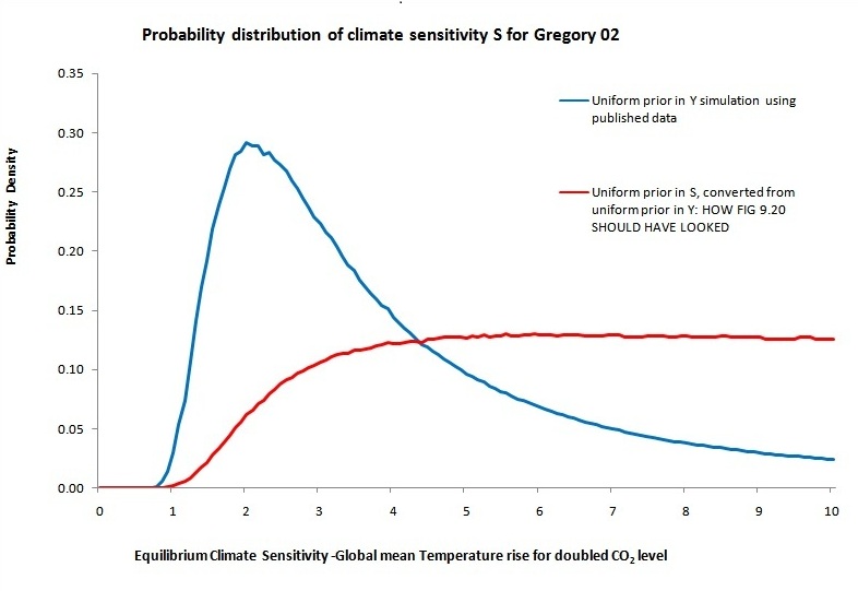
The orange line in Figure 3, below, shows what the Gregory 02 climate sensitivity PDF would have looked like in IPCC Figure 9.20 had it actually been computed on the basis stated in Table 9.3. As you know, that involves multiplying by S2 and renormalizing, reversing out the effect of the multiplication by 3.7/S2 on converting parameter from Y to S. I have computed the PDF using my larger-sample simulation of the Gregory 02 results, as using the transcribed Figure 9.20 graph is not very accurate at high sensitivity levels and the PDF computed from it fluctuates considerably. I have shown the uniform prior in Y based PDF for comparison – the blue line.
Figure 3
I think it a pity that the IPCC failed to show in Figure 9.20 the sensitivity PDF for Gregory 02 on the uniform prior in S basis that the IPCC claimed it was stated on. Had it done so, many more people might have realised just how inappropriate the uniform prior in S basis is. I am not suggesting that the failure to transform the Gregory 02 sensitivity PDF to a uniform prior in S basis, in the way that was done with Forster/Gregory 06, was deliberate. I presume that it was just a simple error. But it is surprising that neither the IPCC writing team nor the paper author realised that the Gregory 02 sensitivity PDF embodied an approximately uniform prior in Y, not in S. That point seemed fairly obvious from reading the paper. And it does raise doubts about how informed was the consent of the Forster/Gregory 06 authors (or at least that of Jonathan Gregory) to the transformation of the results of that paper onto a uniform prior in S basis.
I said earlier that the fact that a substantial portion of the distribution of the estimate for Y was below zero – a physically unrealistic result – suggested that the estimate of Q may be too low and/or the estimate of F too high. And I think that there are grounds for that suspicion. The central value of 0.32 Wm-2 (per unit area of the Earth) for the change in heat flux into the ocean, F, over 1957-1994 was based on the Levitus et al. 2000 dataset. That dataset was corrected in 2005, giving a lower figure of 0.20 Wm-2 (over the same period), or possibly slightly less. The corrections made to the Levitus dataset in 2009 would reduce the ocean heat flux figure further, of course, but that post-dates AR4.
Also, the Gregory 02 central estimate for the total change in forcings between 1861–1900 and 1957–1994 of 0.36 Wm-2 looks on the low side to me. I note that the key Sulphate aerosols component was derived using the HadCM3 AOGCM, rather than being based directly on observational estimates. If one uses instead the well known GISS observational forcings dataset, from 2007, used in NASA GISS model E, the total change in forcings between the two periods is twice as high, at 0.72 Wm-2 [i]. The comparable net change in radiative forcings illustrated in AR4 WG1 Figure 2.23, as used by another GCM, seems to be even higher, at around 1 Wm-2 between 1861–1900 and 1957–1994.
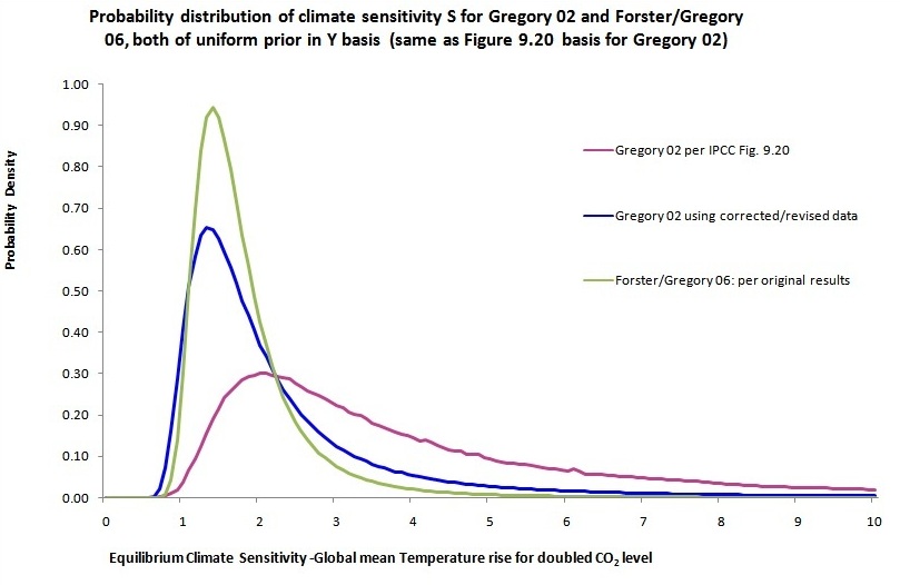
If the corrected 2005 Levitus dataset ocean heat flux data and the GISS change in radiative forcings estimates were used, (Q – F) in the Gregory 02 equation (3) would be centred on 0.68 Wm-2 instead of on 0.20 Wm-2. Recomputing the Gregory 02 results, simply substituting those corrected/revised central estimates for the original ones, would produce a substantially lower estimate of S, with a far thinner upper tail to its PDF – much more in line with the Forster/Gregory 06 results. Figure 4, below, illustrates this. The PDFs are all given on the original, approximately uniform in Y, basis.
Figure 4
I look forward to hearing from you once you and your colleagues have investigated this matter. I appreciate that if you need to call in external statistical expertise, that may take some time.
Yours sincerely
Nicholas Lewis
7 July 2011
[i] This is treating missing 1861-1879 values as the same as for 1880, except for stratospheric (volcanic) aerosols.


Leave A Comment