How inconstant are climate feedbacks – and does it matter?

Originally posted on April 18, 2017 at Climate Etc.

Kyle Armour has a new paper out in Nature Climate Change: “Energy budget constraints on climate sensitivity in light of inconstant climate feedbacks”.

Its two key claims are:

“global climate models robustly show that feedbacks vary over time, with a strong tendency for climate sensitivity to increase as equilibrium is approached. … I find that the long-term value of climate sensitivity is, on average, 26% above that inferred during transient warming within global climate models, with a larger discrepancy when climate sensitivity is high.”

“Moreover, model values of climate sensitivity inferred during transient warming are found to be consistent with energy budget observations, indicating that the models are not overly sensitive. Using model-based estimates of how climate feedbacks will change in the future, in conjunction with recent energy budget constraints, produces a current best estimate of equilibrium climate sensitivity of 2.9 °C (1.7–7.1 °C, 90% confidence). “

I will examine these claims in turn. But first I would like to point out that even if they were both sound (which on my analysis they aren’t), it would be almost entirely irrelevant to the level of temperatures in the final decades of this century, at least in scenarios in which greenhouse gas concentrations continue to rise until then. That is because up to 2100 warming will depend very largely on the level of the transient climate response (TCR), not on equilibrium climate sensitivity (ECS). The claims made by Kyle Armour have no bearing on TCR or on its estimation from warming over the instrumental period.

Armour’s first key claim

The first claim is entirely about the behaviour of atmosphere-ocean global climate models (AOGCMs), specifically the CMIP5 models used in the IPCC AR5 report. As these models take thousands of simulation years to equilibrate, their ECS is usually estimated from the results of a simulation in which atmospheric CO₂ concentration is abruptly quadrupled immediately after the simulation starts (abrupt4xCO2). These simulations start from an equilibrium preindustrial state and usually cover 150 years. The top-of-atmosphere (TOA) radiative imbalance (N) is plotted against the change in global surface temperature (GMST or T), usually as annual means, over the course of the simulation – a so-called “Gregory plot”. Ordinary least-squares (OLS) linear regression is performed on the plot values and ECS (the equilibrium rise in T for a doubling of CO₂) is derived as half the x-intercept.[1]

In AR5 the ECS of CMIP5 models was estimated by Gregory-plot OLS regression over years 1‑150 of abrupt4xCO2 simulations.[2] This method implicitly assumes that aggregate climate feedbacks are constant over time as well as independent of climate state (and hence of whether CO2 concentration is doubled or quadrupled).[3]

However, in about 90% of CMIP5 models, the slope of the Gregory-plot is steeper over the first few decades of the abrupt4xCO2 simulation than subsequently, pointing to net climate feedbacks weakening over time. This has led to an alternative estimate of their ECS, differing only in that the Gregory-plot regression utilizes only years 21-150 of the abrupt4xCO2 simulations, to capture models’ feedbacks after the early decades.[4] Kyle adopts this method for estimating models true ECS values.[5]

Figure 1 shows a Gregory plot for the GFDL-CM3 model, illustrating that the slope of the fitted regression line (representing net climate feedbacks, inclusive of the Planck feedback) is slightly lower, and the resulting ECS estimate slightly higher, using data from years 21-150 rather than 1-150 (and vice versa when using data for years 1-20 rather than 21-150).

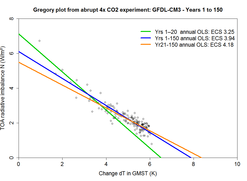
Figure 1: Example Gregory plot with regression line fits. ECS estimates are half the x-intercepts. Values for individual years are marked by open circles; dT generally increases with time.

Armour also estimates the effective radiative forcing (ERF) from a doubling of CO₂ concentration (F_2xCO2) by Gregory plot regression, as half the y-intercept from Gregory-plot regression using years 1-5 of the abrupt4xCO2 simulation data. I think it preferable to use regression over years 1-20 to estimate F_2xCO2, [6] which in line with James Hansen’s finding that 10 to 30 year regression periods were best for this purpose.[7] Doing so gives results broadly in line with estimates based on fixed sea-surface temperature (SST) simulations, the other standard method of estimating ERF.

Kyle Armour then compares the ECS estimates from regression of abrupt4xCO2 simulation data with estimates (called ECS_infer) intended to reflect approximations to ECS derivable when forcing increases gradually, as over the historical period. He derives ECS_infer in models from changes in T, N and forcing (F)[8] over the first 100 years of simulations in which CO₂ concentration rises by 1% per annum (1pctCO2), [9] taking 31-year averages, using the energy budget formula (Δ denoting a change):

ECS_infer = F_2xCO2 * ΔT/( ΔF – ΔN).[10]

However, recent research has confirmed that CO₂ forcing increases slightly faster than logarithmically with concentration,[11] which implies calculating F_2xCO2 as half the value derived from a quadrupling of CO₂ concentration overstates its value (by 4.6% or so).[12]

The paper’s first main result is that ECS is on average 26% higher than ECS_infer in CMIP5 models; Armour also finds that the excess increases with both ECS and ECS_infer.

When I calculate ECS/ECS_infer using Kyle Armour’s F_2xCO2 values, analytical forcing approximations and set of 21 CMIP5 models, I obtain the same 1.26 average ratio.[13]

However, when I use F_2xCO2 values derived, IMO more satisfactorily, from regression over years 1-20 of abrupt4xCO2 data rather than years 1-5, and estimates of CO₂ forcing that allow for its slightly faster than logarithmic relationship with concentration, the mean ECS/ECS_infer ratio falls to 1.20. When I include all 33 CMIP5 models for which I have data, the average ratio reduces further, to 1.16.

The distribution of the ECS/ECS_infer ratio is quite skewed; as Kyle Armour reports, it rises with ECS. For models with an ECS of 3°C or less, the average ratio is only 1.07. It is generally considered appropriate to use the median rather than the mean as a central measure for skewed distributions.[14] The average is inflated by an extremely high ECS/ECS_infer ratio for the highly sensitive CSIRO-Mk3-6-0 model. The median ECS/ECS_infer ratio is only 1.12, under half Kyle’s 1.26 average value.

Even if ECS were as high as it is in the median CMIP5 model (3.2°C), using instead the ECS_infer value of 3.2 / 1.12 = 2.86°C when projecting warming over the next century or two would make very little difference on non-mitigation or strong mitigation scenarios. Armour’s results end to support this, at least over the next century, in that they show that ECS/ECS_infer changes very slowly over time under (1% p.a.) CO₂ ramping.[15]

There is as yet no observational evidence that climate sensitivity increases with time in the real climate system – although this cannot be ruled out – nor is it fully understood why it increases in most AOGCMs. In any event, even if real-world climate sensitivity does increase with time, in the longer run other factors that are not reflected in ECS, such as melting ice sheets, are probably more important. Therefore, while time-varying climate sensitivity is of considerable interest from a theoretical point of view, for practical purposes its influence is likely to be very modest.

Armour’s second key claim

It does not follow, from model values of climate sensitivity inferred during transient warming being are found to be “consistent” with energy budget observations, that in general the models are not overly sensitive.[16] By “consistent” Kyle Armour means that the 5-95% uncertainty range of observationally-based energy budget ECS estimates spans the full CMIP5 model range of ECS_infer. This is broadly true, but of limited relevance.

What is much more important is whether the two distributions are concentrated around values close to each other or not. For both our sets of CMIP5 models, I calculate the median (and mean) ECS_infer value as 3.0°C.[17] This is well above median estimates, of ECS_infer as a proxy for ECS, from the highest quality energy budget studies based on warming over the historical period: Otto et al. 2013’s best two estimates were 1.9 to 2.0°C. Lewis and Curry 2015’s median estimates, based on IPCC AR5 forcing and heat uptake data, were all 1.6°C or 1.7°C, depending on period used. An update I blog-published last year gave a median ECS estimate of 1.74°C. If the globally-complete Cowtan & Way infilled version of the HadCRUT4 surface temperature dataset is used instead of the original, this ECS estimate becomes 1.9°C. This is a long way below the median CMIP5 ECS_infer value of 3.0°C.

Armour’s 2.9°C ECS best estimate (although not the uncertainty range) is obtainable simply by (a) scaling up the ECS_infer value resulting from applying the energy budget formula to the Otto et al. observational constraints, being 1.99°C, by the 24% adjustment factor for ΔT that Richardson et al. (2016) derives, giving an ECS_infer estimate of 2.47°C (which agrees to Armour’s Table 1, first row); and then (b) multiplying by 1.1945, the fitted ratio of ECS/ECS_infer per Armour’s equation (5), which relates the ECS/ECS_infer ratio to the value of ECS_infer.

I don’t accept that the Richardson et al. 24% warming adjustment is realistic; see my critique of that study here. Moreover, Armour’s equation (5) is actually of little use in estimating how ECS/ECS_infer varies with ECS_infer; for his set of CMIP5 models the equation (5) fitted values explain only 4% of the variance in ECS/ECS_infer.

I’m not in any event sure how useful it is to produce a best estimate of ECS (as opposed to ECS_infer) from instrumental period observational data, since not only can ECS/ECS_infer only be estimated in AOGCMs but the ratio varies widely between different AOGCMs.

Conclusions

I like Kyle Armour and respect him as a scientist, but I think this paper’s primary finding is greatly overstated and that applying it using the questionable Richardson et al. 24% adjustment to warming measured by HadCRUT4 does not produce a very meaningful secondary finding.

It has in fact been found that when CMIP5 models are forced with specified SST anomalies matching the pattern of warming over the historical period, they produce net climate feedbacks of the order of 2 Wm^-2K^-1, closely consistent with the modest ECS best estimates from good observationally-based energy budget studies.[18] The real questions seem to be why do AOGCMs simulate very different warming patterns under increased CO2 concentration than those that have actually occurred during the historical period, and why do their net feedback strengths differ so much between these warming patterns.

Acknowledgements

Kyle Armour kindly shared the final version of his paper with me earlier, thus facilitating my analysis and enabling us to have a useful discussion about his paper and my analysis. Kyle Armour has seen an earlier draft of this article and, although he does not concur with the choices that I have made in my analysis, he has provided helpful comments.

Nicholas Lewis

Notes and references

[1] The logic here is that when N is zero the model will have reached equilibrium, and that CO₂ forcing is logarithmically related to its concentration so that forcing from a quadrupling of CO₂ concentration is twice that from a doubling.

[2] AR5 Table 9.5 used ECS values from Andrews, T., et al. “Forcing, feedbacks and climate sensitivity in CMIP5 coupled atmosphere-ocean climate models.” Geophysical Research Letters 39.9 (2012) and Forster, Piers M., et al. “Evaluating adjusted forcing and model spread for historical and future scenarios in the CMIP5 generation of climate models.” Journal of Geophysical Research: Atmospheres 118.3 (2013): 1139-1150.

[3] It also assumes, by the use of OLS regression, that internal variability in the regressor variable T is small enough to be ignored. It further assumes that T and N (a) have been correctly adjusted by deducting their equilibrium absolute levels in preindustrial conditions; (b) that any drift in those levels is constant over time and has been correctly adjusted for; and (c) that any imbalance in N in equilibrium, due e.g. to energy leakage in the model, is independent of the model’s climate state. Estimation of ECS by running the simulation until equilibrium is also dependent on assumptions (b) and (c).

[4] Andrews, T. JM Gregory, and MJ Webb. “The dependence of radiative 892 forcing and feedback on evolving patterns of surface temperature change in climate models.” Journal of Climate 28.4 (2015): 1630-1648.

[5] Although Kyle Armour twice states in the paper (Methods) that he estimates model ECS by regression over years 121-150 of abrupt4xCO2 simulations, he has confirmed to me that this is an error and that he actually used regression over years 21-150. The ECS values in Supplementary Table 1 are fairly closely in line with my own estimates from regressing over years 21-150.

[6] During year 1, the initial instantaneous radiative forcing reduces to reach ERF, as stratospheric, tropospheric and fast land surface adjustments (such as CO2-induced stomatal closure, which reduces evapotranspiration and affects soil moisture) to the increase in CO₂ concentration, unrelated to surface temperature, take place. Accordingly, including year 1 in a regression to estimate F_2xCO2 does not produce pure ERF estimation. Year 1, which often lies above the years 1-20 regression line, has a much larger impact on 5 year regression. Years 1-5 regression estimates are accordingly usually rather higher than year 1-20 estimates, on average by 5% for the 34 CMIP5 models that I have abrupt4xCO2 data for (by 7% for the subset of 21 models studied by Kyle Armour). Regression over years 1-5 is also much more affected by interannual variability. The mean and median CO₂ ERF in CMIP5 models derived by regression over years 1-20 lies between that estimated from regression over years 2-5 and 2-10, before any material change in model’s net climate feedback occurs.

[7] Hansen, J., et al. “Efficacy of climate forcings.” Journal of Geophysical Research: Atmospheres 110.D18 (2005).

[8] Armour states in the paper that he uses an analytical approximation for forcing as time t years into the 1pctCO2 simulation: ΔF(t) = F_2xCO2 *t/69, which would marginally overstates ΔF (and hence understate ECS infer) even if the underlying assumption that CO₂ forcing increases exactly logarithmically with forcing is correct; the doubling time for a 1% per annum rate of increase is 69.7 years. In fact, he used a divisor of 70 years, not 69 years (pers. comm.), which has a opposite but milder effect, but which appears to be cancelled out by his similarly taking the mean value for t as 100 years rather than the exact 99.5 years.

[9] I generally use regression over years 1-30 of abrupt4xCO2 simulations to estimate ECS as inferred from historical warming, as the signal-to-noise ratio is much higher in abrupt4xCO2 simulations than in 1pctCO2 simulations. Doing so fairly reflects the circa 30 year weighted average period since each year’s forcing increment arose. On average, the resulting estimates are within 1% of those I estimate from 1pctCO2 simulations on the same basis that Kyle Armour uses.

[10] The paper uses the change ΔQ in the rate of increase in global heat content rather than ΔN, but these two variables have virtually identical values in the real world, and should do in AOGCMs.

[11] Byrne, B., and C. Goldblatt. “Radiative forcing at high concentrations of well‐mixed greenhouse gases.” Geophysical Research Letters 41.1 (2014): 152-160; Etminan, M., et al. “Radiative forcing of carbon dioxide, methane, and nitrous oxide: A significant revision of the methane radiative forcing.” Geophysical Research Letters (2016).

[12] Assuming CO₂ is the only greenhouse gas being increased. At year 100 of the 1pctCO2 simulations, when CO₂ concentration has increased by a factor of 2.7, the ratio of CO₂ forcing to its level when its concentration it quadrupled is ~2% short of a logarithmic relationship.

[13] This is so whether using his Supplementary Table 1 ECS values or those I calculate myself from Gregory-plot regression over years 21-150. All of my ECS_infer values are within 2% of his, save for one that is 5% lower.

[14] This issue was considered by the AR5 authors in relation to observational estimates of ECS, which also have skewed distributions; they likewise favoured use of the median rather than of the mean.

[15] Armour quantifies this in the final paragraph of the Methods section.

[16] Moreover, Armour bases this claim on a CMIP5 range for ECS_infer of 2.1-3.8°C, whereas on my calculations the range is 2.1-4.4°C, or 2.0-4.4°C taking all 33 models.

[17] On my calculation basis but adjusting the CO2 forcing non-logarithmic factor for appropriate comparison with observationally-based ECS estimates rather than halved estimate of equilibrium warming in abrupt4xCO2 simulation.

[18] Gregory, J. M., and T. Andrews. “Variation in climate sensitivity and feedback parameters during the historical period.” Geophysical Research Letters 43.8 (2016): 3911-3920.

JC note: Peter Fairley in EnergyWise has a good write up on the article, quoting both Kyle and Nic: Will Earth’s Climate Get More Sensitive to CO2? Only Better Satellites Can Say.