Originally posted on Apr 20, 2015 – 4:25 PM at Climate Audit
In Part 1 I introduced the talk I gave at Ringberg 2015, explained why it focussed on estimation based on warming over the instrumental period, and covered problems relating to aerosol forcing and bias caused by the influence of the AMO. In Part 2 I dealt with poor Bayesian probabilistic estimation and summarized the state of observational, instrumental period warming based climate sensitivity estimation. In this third and final part I discuss arguments that estimates from that approach are biased low, and that GCM simulations imply ECS is higher, partly because in GCMs effective climate sensitivity increases over time. I’ve incorporated one new slide here to help explain this issue.
Slide 19
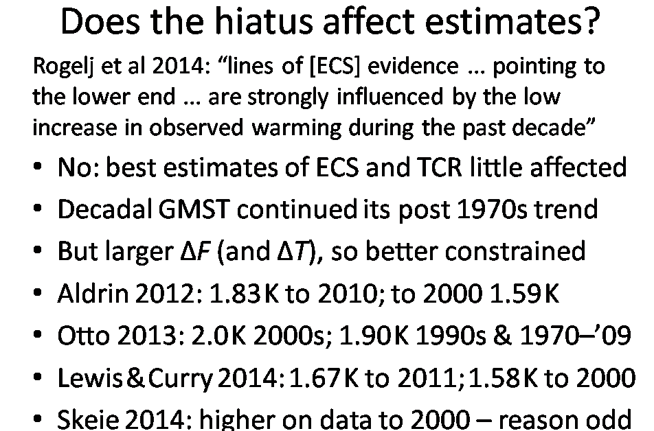
I’ll start with an easy target: claims that reduced instrumental period warming based ECS estimates that have been published over the last few years reflected the hiatus in warming over the last decade. Such claims are demonstrably false. The main effect of using data extending past 2000 is to provide better constrained ECS estimates, as the anthropogenic signal rose further above background noise.
Most recent studies that give results using data for different periods actually show lower, not higher, ECS median estimates when data extending only to circa 2000 is used. Skeie 2014 is an exception. I attribute this to the less strong observational constraints available from such data being unable to counteract its excessively negative aerosol forcing prior distribution.
Slide 20
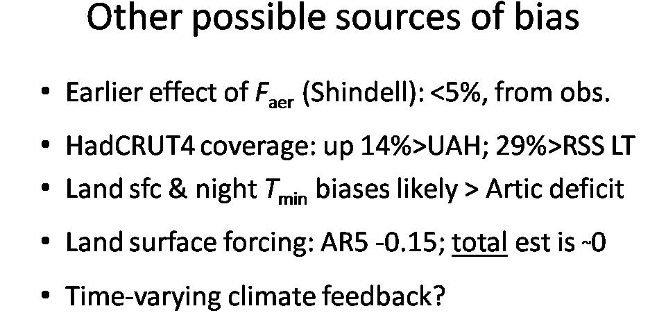
Now for some genuine issues. First, in a 2014 paper Drew Shindell argued that inhomogeneous forcing, principally by aerosols, with a greater concentration in the northern hemisphere – particularly in the extratropics – than homogenous GHG forcing would have a greater effect on transient global warming. That is principally because the northern hemisphere has more land and warms more rapidly. That aerosol forcing reached a peak level some time ago, unlike for GHGs, also contributes to the effect. The result would be that TCR, and hence ECS, estimates based on observed global warming were biased down.
I think there is in principle something in Shindell’s argument, but I regard his GCM-based estimate of the magnitude of the bias as absurdly high. Based on a simple model and observational constraints as to the ratios of transient warming for various latitude zones, I obtain a best estimate for the bias of no more than about 5%. It would be difficult to reconcile a significant bias with estimates from the non-energy budget ‘good’ studies being in line with energy-budget based estimates. Good non energy-budget studies should be unaffected by this issue due to their use of models that resolve forcing and temperature by hemisphere, and within each hemisphere by latitude zone and/or land vs ocean.
In his Ringberg talk, Gavin Schmidt stated that in the GISS-E2-R AOGCM, the transient responses (over ten years) to aerosol forcing and land use were respectively 1.33x and 3.65x as large as that to GHG forcing. From this he deduced that TCR and ECS estimated from the model’s historical run were biased low by about 20% and 30% respectively. Picking (over high) median estimates based on historical period unadjusted forcing, of 1.6°C for TCR and 1.9°C for ECS, he claims that these go up by respectively 35% and 60% when adjusted for forcing-specific ‘transient efficacy’.
I am at a loss to understand how the diagnosed increases of 20% and 30% turned into claimed increases of 37% and 63% – maybe this was achieved by using uniform priors. Moreover, the very large estimated land use forcing transient efficacy shown in Gavin Schmidt’s slide is based on an unphysical regression line that implies a very large GMST increase with zero land use forcing. In view of these oddities the findings shown seem questionable.
If, despite my doubts, the results Gavin Schmidt presented are correct for the GISS-E2-R model, they would support Drew Shindell’s argument in relation to that model. But it would not follow that similar biases arise in other models or in the real world. I am aware of only two other AOGCMs for which transient efficacies have been likewise been diagnosed using single-forcing simulations (Shindell 2014 used the standard CMIP5 simulations, which is much less satisfactory). One of those models shows a significantly lower transient efficacy for aerosol forcing than for GHG (Ocko et al 2014), behaviour that implies TCR and ECS estimates based on historical warming would be biased up, not down. The other model also appears to show that behaviour, albeit based only on preliminary analysis.
In the light of the available evidence, I think it very doubtful that aerosol and land use forcing have caused a significant downwards bias in observationally-based estimation of TCR or ECS.
The next two bullet points in slide 20 concern arguments that the widely-used HadCRUT4 surface temperature dataset understates the historical rise in GMST. However, over the satellite era, which provide lower troposphere temperature estimates with virtually complete coverage, HadCRUT4 shows a larger global mean increase than does UAH and, even more so, RSS. It seems quite likely that upward biases arising from land surface changes (UHI, etc.) and the destabilisation of the nocturnal boundary layer (McNider et al 2012) exceed any downwards bias resulting from a deficit of coverage in the Arctic.
For land surface changes, AR5 gives a negative best estimate for albedo forcing but states that overall forcing is as likely positive as negative. On that basis it is inappropriate to include negative land surface forcing values when estimating TCR and ECS from historical warming. Those studies (probably the majority) which include that forcing will therefore tend to slightly overestimate TCR and ECS.
The final point in this slide concerns the argument, put quite strongly at Ringberg (e.g., see here) that climate feedback strength declines over time, so that ECS – equilibrium climate sensitivity – exceeds the effective climate sensitivity approximation to it estimated from changes in GMST, forcing and radiative imbalance (or its counterpart, ocean etc. heat uptake) over the instrumental period. As explained in Part 1, in many but not all CMIP5 models global climate feedback strength declines over time, usually starting about 20-30 years after the (GHG) forcing is imposed. I address this issue in the next slide.
Slide 21
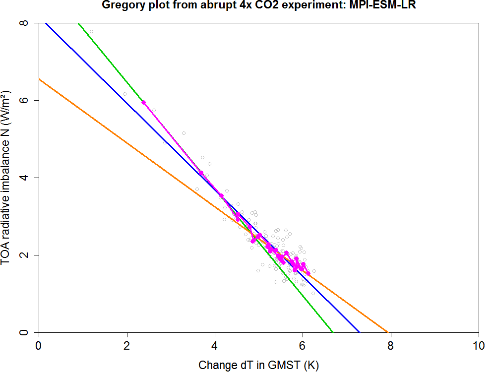
As running AOGCMs to equilibrium takes so long, their ECS values are generally diagnosed by regressing their top of atmosphere (TOA) radiative imbalance N – the planetary heat absorption rate – on dT, their rise in GMST, during a period of, typically, 150 years following a simulated abrupt quadrupling in CO2 concentration. The regression line in such a ‘Gregory plot’ is extrapolated to N = 0, indicating an equilibrium state. ECS is given by half the dT value at the N = 0 intercept. That is because CO2 forcing increases logarithmically with concentration, and a quadrupling equates to two doublings.
Slide 21, not included in my Ringberg talk, illustrates the potential bias in estimating ECS from observed warming over the instrumental period. It is a Gregory plot for the MPI-ESM-LR model (chosen in honour of the Ringberg hosts). The grey open circles show annual mean data, that closest to the top LH corner being for year 1. The magenta blobs and line show pentadal mean data, which I have used to derive linear fits (using ordinary least squares regression). The curvature in the magenta line (a reduction in slope after about year 30) indicates that climate feedback strength (given by the slope of the line) is decreasing over time.
CMIP5 model ECS values given in AR5 were based on regressions over all 150 years of data available, as for the blue line in the slide. I have compared ECS values estimated by regressing over years 21-150 (orange line), as in Andrews et al (2014), with ECS values estimated from the first 35 years (green line). Since the growth in forcing to date approximates to a 70-year linear ramp, and at the end of a ramp the average period since each year’s increase in forcing is half the ramp period, 35 years from an abrupt forcing increase is fairly representative of the observable data. As can be seen, the ECS estimate implied by the orange years 21-150 regression line is higher than that implied by the blue year 1-150 regression line, which in turn exceeds that implied by the green years 1-35 regression line. This indicates an increase over time in effective climate sensitivity.
On average, ECS diagnosed for CMIP5 models by regressing over years 21-150 of their abrupt 4x CO2 Gregory plots exceeds that diagnosed from years 1-35 data by 19%. However, excluding models with a year 21-150 based ECS exceeding 4°C reduces the difference to 12%. This is fairly minor. The difference is not nearly large enough to reconcile the best estimates of ECS from observed warming over the instrumental period with most CMIP5 model ECS values. And it is not relevant to differences between observationally-based TCR estimates and generally higher AOGCM TCR values.
It is, moreover, unclear that higher AOGCM ECS values diagnosed by Gregory plot regression over years 21-150 are more realistic than those starting from year one. Andrews et al (2014) showed, by running the HadGEM2-ES abrupt 4x CO2 simulation for 1290 years (to fairly near equilibrium), that the ECS diagnosed for it from regressing over years 21-150 appears to be substantially excessive. The true model ECS appears to be closer to the estimate based on regressing over years 1-35, which is 27% lower.
Importantly, an increase in effective climate sensitivity over time, if it exists, is almost entirely irrelevant when considering warming from now until the final decades of this century. The extent of such warming, for a given increase in GHG levels, is closely dependent on TCR, irrespective of ECS. Even if effective climate sensitivity does increase over time, that would not bias estimation of TCR from observed historical warming. And the projected effect on warming from effective climate sensitivity increasing in line with a typical CMIP5 model would be small even over 300 years – only about 5% for a ramp increase in forcing, if one excludes HadGEM2-ES and the Australian models (two of which are closely related to it, with the third being an outlier).
Slide 22
Although the increase in effective climate sensitivity, due to a reduction in climate feedback strength, with time in many CMIP5 models appears to have little practical importance, at least on a timescale of up to a few centuries, finding out why it occurs is relevant to gaining a better scientific understanding of the climate system.
In a model-based study, Andrews et al (2014) linked the time-variation to changing patterns of sea-surface temperature (SST), principally involving the tropical Pacific. In current AOGCMs, after an initial delay of a few years, on a multidecadal timescale the eastern tropical Pacific warms significantly more than the western part and the tropical warming pattern becomes more El-Nino like, affecting cloud feedback.
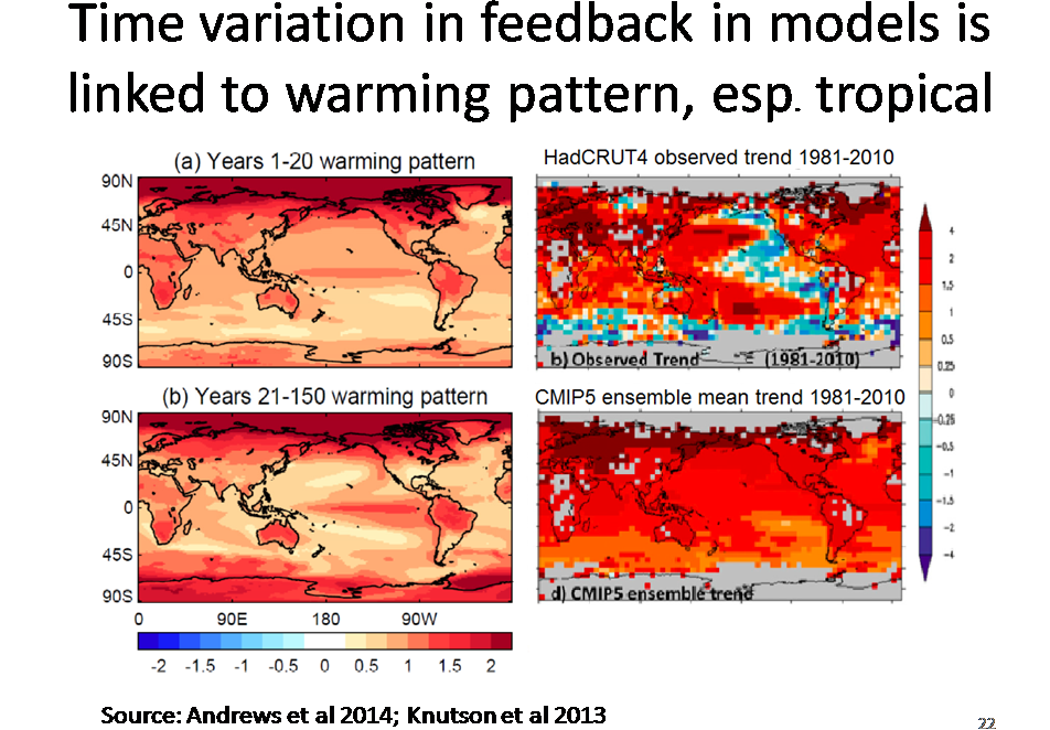
The two LH panels in slide 22, from Tim Andrews’ paper and talk, show the CMIP5 model ensemble mean patterns of surface warming during the first 20 and the subsequent 130 years after an abrupt quadrupling of CO2. The colours show the rate of local increase relative to that in GMST. It can be seen that even during the first 20 years, warming is strongly enhanced across the equatorial Pacific.
The RH panels, taken from a different paper, show observed and modelled patterns of warming over 1981–2010. The CMIP5 ensemble mean trend (bottom RH panel) shows a pattern in the tropical Pacific fairly consistent with that over the first 20 years of the abrupt 4x CO2 experiment, as one might expect. But the observed trend pattern (top RH panel) is very different, with cooling over most of the eastern tropical Pacific, including the equatorial part.
So observations to date do not appear consistent with the mean evolution of eastern tropical Pacific SST predicted by CMIP5 models. Given Tim Andrew’s finding that weakening of climate feedback strength over time in CMIP5 models is strongly linked to evolving eastern tropical Pacific SST patterns, that must cast considerable doubt on whether effective climate sensitivity increases over time in the real world.
Slide 23
There are other reasons for doubting the realism of the changing SST patterns in CMIP5 models that Andrews et al (2014) found to be linked to increasing climate sensitivity.
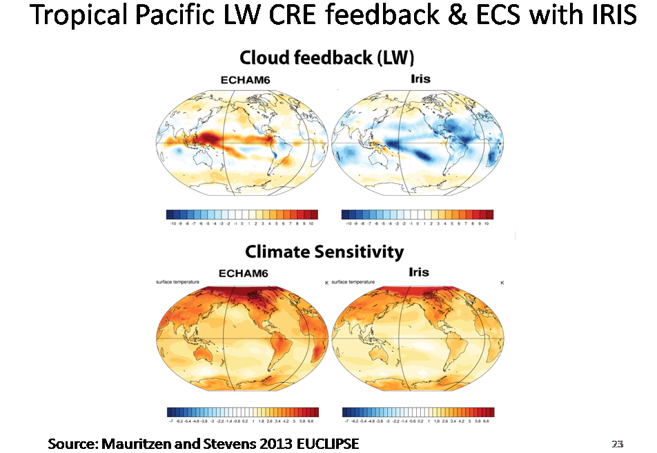
The strong warming in the deep tropics across the Pacific over years 21–150 is linked to positive longwave (LW) cloud feedback, which in CMIP5 models strengthens and spreads further after years 1–20. But is this behaviour realistic? In parallel with MPI’s main new CMIP6 model MPI-ESM2 (ECHAM6 plus an ocean module), Thorsten Mauritzen has been developing a variant with a LW iris, an effect posited by Dick Lindzen some years ago (Lindzen et al 2001). The slides for Thorsten Mauritzen’s Ringberg talk, which explained the Iris variant and compared it with the main model, are not available, but slide 23 comes from a previous talk he gave about this work. It shows the equilibrium position; so far only simulations by the fast-equilibrating slab-ocean version of the Iris model have been run. [Note: the related paper, Mauritsen and Stevens 2015, has now been published.]
As the top panels show, unlike the main ECHAM6/MPI-ESM2 model, the Iris version exhibits no positive LW cloud feedback in the deep tropical Pacific. And the bottom panels show that, accordingly, warming in the central and eastern tropical Pacific remains modest. This suggests that, if the Iris effect is real, any increase in effective climate sensitivity over time would likely be much lower than CMIP5 model ensemble mean behaviour implies. The Iris version also has a lower ECS than the main model, although not as low as might be expected from the difference in LW cloud feedback, as this is partially offset by a more positive SW cloud feedback.
Slide 24
Slide 24 lists methods of estimating ECS other than those based on observed multidecadal warming. I explained in Part 1 that I concurred with AR5’s conclusions that estimating ECS from short term responses involving solar or volcanic forcing or TOA radiation changes was unreliable, and that true uncertainty in paleoclimate estimates was larger than for instrumental period warming based estimates. That implies that combining paleo ECS estimates with those based on instrumental period warming would not change the latter very much.
I also showed, in Part 2, that the model most widely used for Perturbed Physics/Parameter Ensemble studies, HadCM3/SM3, could not successfully be constrained by observations of mean climate and/or climate change, and so was unsuitable for use in estimating ECS or TCR. (Such use nevertheless underlies UKCP09, the official UK 21st century climate change projections.)
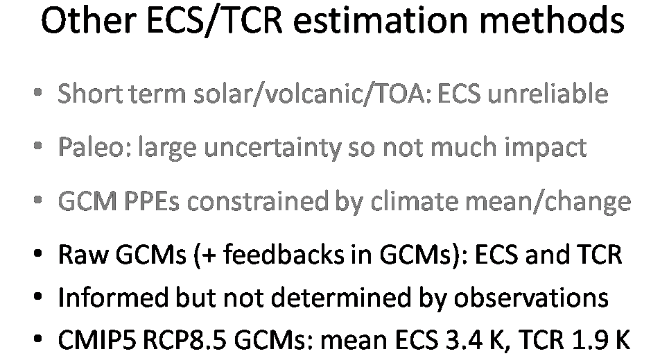
The other main source of ECS estimates involves GCMs more directly. Distributions for ECS and TCR can be derived from estimated model ECS and actual model TCR values. A 5-95% ECS range for CMIP5 models, of 2–4.5°C, was given in Figure 1, Box 12.2 of AR5. Feedbacks exhibited by GCMs can also be analysed, and to some extent compared with observations. But although development of GCMs is informed by observations, their characteristics are not determined by observational constraints. If the climate system were thoroughly understood and AOGCMs accurately modelled its physical processes on all scales that mattered, one would expect all aspects of their behaviour to be fairly similar, and the ECS and TCR values they exhibited might then be regarded as reliable estimates. However, those requirements are far from being satisified.
Since AOGCMs tend to be similar in many respects, it is moreover highly doubtful that a statistically-valid uncertainty range for ECS or TCR can be derived from CMIP5 model ECS and TCR values. If some key aspect of climate system behaviour is misrepresented in (or unrepresented by) one CMIP5 model, the same problem is likely to be common to many if not all CMIP5 models.
In this connection, I’ll finish by highlighting two areas relevant to climate sensitivity where model behaviour seems unsatisfactory across almost all CMIP5 models.
Slide 25
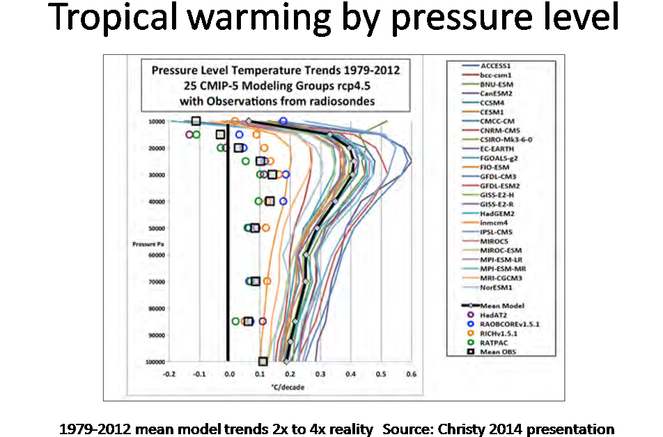
Slide 25 compares tropical warming by pressure level (altitude) in CMIP5 models and radiosonde observations over 1979-2012. Most models not only show excessive near-surface warming, by a factor of about two on average, but a much greater increase with height than observations indicate. This is the ‘missing hot-spot’ problem. The ratio of tropical mid-troposphere to surface warming would be expected to be smaller in a model with a LW iris than in one that does not, a point in favour of such a feature.
Figure 9.9 in AR5 showed much the same discrepancy – an average factor of about 3x – between observed and modelled temperature trends in the tropical lower troposphere over 1988-2012. Observations in that case were based on satellite MSU datasets and reanalyses that used models to assimilate data.
Slide 26
A lot of the discussion at Ringberg 2015 concerned clouds, one of the most important and least well understood elements of the climate system. Their behaviour significantly affects climate sensitivity.
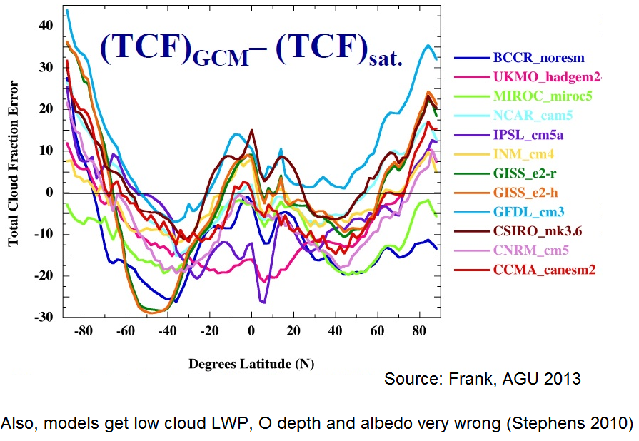
Slice 26 shows errors in cloud fraction by latitude for twelve CMIP5 GCMs. (TCF)sat. is the average per MODIS and ISCCP2 observations. It can be seen that most models have too little cloud cover in the tropics and, particularly southern, mid latitudes, and too much at high latitudes. Errors of this magnitude indicate that reliance should not be placed on cloud feedbacks exhibited by current climate models.
Models also appear to have excessive low cloud liquid water path, optical depth and albedo, which may result in negative optical depth climate feedback being greatly underestimated in models (Stephens 2010).
Slide 27
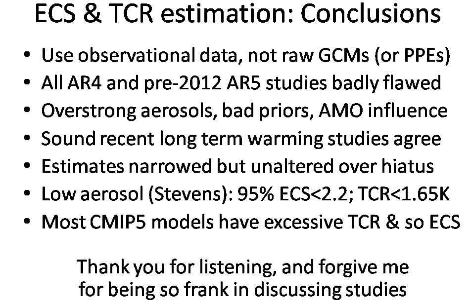
My concluding slide reiterates some of the main points in my talk. Assuming Bjorn Stevens’ revised estimate of aerosol forcing is correct, then the 95% uncertainty bounds on ECS and TCR from observed multidecadal warming are well below the mean ECS and TCR values of CMIP5 models. It will be very interesting to see how these discrepancies between models and observations are resolved, as I think is likely to occur within the next decade.
Nicholas Lewis
Additional references
Timothy Andrews, Jonathan M. Gregory, and Mark J. Webb (2015): The Dependence of Radiative Forcing and Feedback on Evolving Patterns of Surface Temperature Change in Climate Models. J. Climate, 28, 1630–1648
Lindzen, RS, M-D Chou, AY Hou (2001) Does the Earth have an adaptive infrared iris? Bull. Amer. Meteor. Soc. 82, 417-432, 2001
Mauritsen, T and B Stevens (2015) Missing iris effect as a possible cause of muted hydrological change and high climate sensitivity in models. Nature Geoscience doi:10.1038/ngeo2414
McNider, R. T., et al. (2012) Response and sensitivity of the nocturnal boundary layer over land to added longwave radiative forcing. J. Geophys. Res., 117, D14106.
Ocko IB, V Ramaswamy and Y Ming (2014) Contrasting Climate Responses to the Scattering and Absorbing Features of Anthropogenic Aerosol Forcings J. Climate, 27, 5329–5345
Rogelj J, Meinshausen M, Sedlácek J, Knutti R (2014) Implications of potentially lower climate sensitivity on climate projections and policy. Environ Res Lett 9. doi:10.1088/1748-9326/9/3/031003
Shindell, DT (2014) Inhomogeneous forcing and transient climate sensitivity. Nature Clim Chg: DOI: 10.1038/NCLIMATE2136
Stephens, GL (2010) Is there a missing low cloud feedback in current climate models? GEWEX News, 20, 1, 5-7.
Update 21 April 2015
The Mauritsen and Stevens paper about the new MPI Iris model has just been published. I have added a reference to it, and to a couple of inadvertently omitted references.
Leave A Comment