Originally a post on December 19, 2012 at Bishop Hill
There has been much discussion on climate blogs of the leaked IPCC AR5 Working Group 1 Second Order Draft (SOD). Now that the SOD is freely available, I can refer to the contents of the leaked documents without breaching confidentiality restrictions.
I consider the most significant – but largely overlooked – revelation to be the substantial reduction since AR4 in estimates of aerosol forcing and uncertainty therein. This reduction has major implications for equilibrium climate sensitivity (ECS). ECS can be estimated using a heat balance approach – comparing the change in global temperature between two periods with the corresponding change in forcing, net of the change in global radiative imbalance. That imbalance is very largely represented by ocean heat uptake (OHU).
Since the time of AR4, neither global mean temperature nor OHU have increased, while the IPCC’s own estimate of the post-1750 change in forcing net of OHU has increased by over 60%. In these circumstances, it is extraordinary that the IPCC can leave its central estimate and ‘likely’ range for ECS unchanged.
I focussed on this point in my review comments on the SOD. I showed that using the best observational estimates of forcing given in the SOD, and the most recent observational OHU estimates, a heat balance approach estimates ECS to be 1.6–1.7°C – well below the ‘likely’ range of 2–4.5°C that the SOD claims (in Section 10.8.2.5) is supported by the observational evidence, and little more than half the best estimate of circa 3°C it gives.
The fact that ECS, as derived using the new aerosol forcing estimates and a heat balance approach, appears to be far lower than claimed in the SOD is highlighted in an article by Matt Ridley in the Wall Street Journal, which uses my calculations. There was not space in that article to go into the details – including the key point that the derived ECS estimate is very well constrained – so I am doing so here.
How does the IPCC arrive at its estimated range for climate sensitivity?
Methods used to estimate ECS range from:
(i) those based wholly on simulations by complex climate models (GCMs), the characteristics of which are only very loosely constrained by climate observations, through
(ii) those using simpler climate models whose key parameters are intended to be constrained as tightly as possible by observations, to
(iii) those that rely wholly or largely on direct observational data.
The IPCC has placed a huge emphasis on GCM simulations, and the ECS range exhibited by GCMs has played a major role in arriving at the IPCC’s 2–4.5°C ‘likely’ range for ECS. I consider that little credence should be given to estimates for ECS derived from GCM simulations, for various reasons, not least because there can be no assurance that any of the GCMs adequately reflect all key climate processes. Indeed, since in general GCMs significantly overestimate aerosol forcing compared with observations, they need to embody a high climate sensitivity or they would underestimate historical warming and be consigned to the scrapheap. Observations, not highly complex and unverifiable models, should be used to estimate the key properties of the climate system.
Most observationally-constrained studies use instrumental data, for good reason. Reliance cannot be placed on paleoclimate proxy-based estimates of ECS – the AR4 WG1 report concluded (Box 10.2) that uncertainties in Last Glacial Maximum studies are just too great, and the only probability density function (PDF) for ECS it gave from a last millennium proxy-based study contained little information.
Because it has historically been difficult to estimate ECS purely from instrumental observations, a standard estimation method is to compare observations of key observable climate variables, such as zonal temperatures and OHU, with simulations of their evolution by a relatively simple climate model with adjustable parameters that represent, or are calibrated to, ECS and other key climate system properties. A number of such ‘inverse’ studies, of varying quality, have been performed; I refer later to various of these. But here I estimate ECS using a simple heat balance approach, which avoids dependence on models and also has the advantage of not involving choices about niceties such as truncation parameters and Bayesian priors, which can have a major impact on ECS estimation.
Aerosol forcing in the SOD – a composite estimate is used, not the best observational estimate
Before going on to estimating ECS using a heat balance approach, I should explain how the SOD treats forcing estimates, in particular those for aerosol forcing. Previous IPCC reports have just given estimates for radiative forcing (RF). Although in a simple world this could be a good measure of the effective warming (or cooling) influence of every type of forcing, some forcings have different efficacies from others. In AR5, this has been formalised into a measure, adjusted forcing (AF), intended better to reflect the total effect of each type of forcing. It is more appropriate to base ECS estimates on AF than on RF.
The main difference between the AF and RF measures relates to aerosols. In addition, the AF uncertainty for well-mixed greenhouse gases (WMGG) is double that for RF. Table 8.7 of the SOD summarises the AR5 RF and AF best estimates and uncertainty ranges for each forcing agent, along with RF estimates from previous IPCC reports. The terminology has changed, with direct aerosol forcing renamed aerosol-radiation interactions (ari) and the cloud albedo (indirect) effect now known as aerosol-cloud interactions (aci).
Table 8.7 shows that the best estimate for total aerosol RF (RFari+aci) has fallen from −1.2 W/m² to −0.7 W/m² since AR4, largely due to a reduction in RFaci, the uncertainty band for which has also been hugely reduced. It gives a higher figure, −0.9 W/m², for AFari+aci. However, −0.9 W/m² is not what the observations indicate: it is a composite of observational, GCM-simulation/aerosol model derived, and inverse estimates. The inverse estimates – where aerosol forcing is derived from its effects on observables such as surface temperatures and OHU – are a mixed bag, but almost all the good studies give a best estimate for AFari+aci well below −0.9 W/m²: see Appendix 1 for a detailed analysis.
It cannot be right, when providing an observationally-based estimate of ECS, to let it be influenced by including GCM-derived estimates for aerosol forcing – a key variable for which there is now substantial observational evidence. To find the IPCC’s best observational (satellite-based) estimate for AFari+aci, one turns to Section 7.5.3 of the SOD, where it is given as −0.73 W/m² with a standard deviation of 0.30 W/m². That is actually the same as the Table 8.7 estimate for RFari+aci, except for the uncertainty range being higher. Table 8.7 only gives estimated AFs for 2011, but Figure 8.18 gives their evolution from 1750 to 2010, so it is possible to derive historical figures using the recent observational AFari+aci estimate as follows.
The values in Figure 8.18 labelled ‘Aer-Rad Int.’ are actually for RFari, but that equals the purely observational estimate for AFari (−0.4 W/m² in 2011), so they can stand. Only the values labelled ‘Aer-Cld Int.’, which are in fact the excess of AFari+aci over RFari, need adjusting (scaling down by (0.73−0.4)/(0.9−0.4), all years) to obtain a forcing dataset based on a purely observational estimate of aerosol AF rather than the IPCC’s composite estimate. It is difficult to digitise the Figure 8.18 values for years affected by volcanic eruptions, so I have also adjusted the widely-used RCP4.5 forcings dataset to reflect the Section 7.5.3 observational estimate of current aerosol forcing, using Figure 8.18 and Table 8.7 data to update the projected RCP4.5 forcings for 2007–2011 where appropriate. The result is shown below.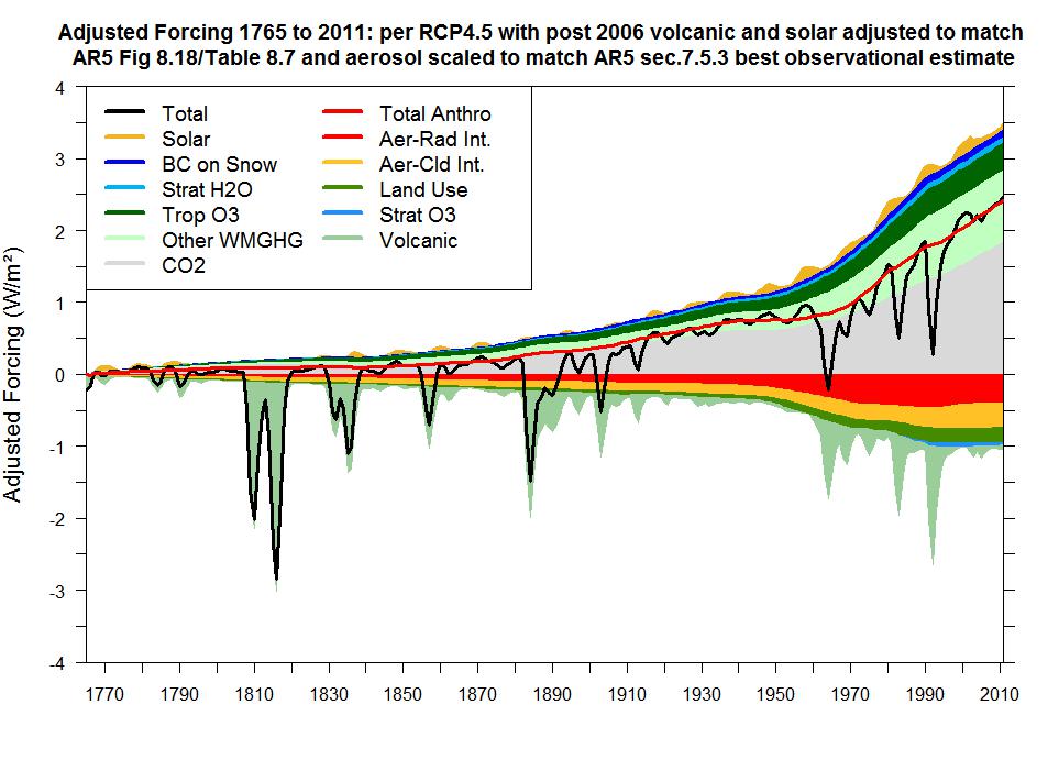 The adjustment I have made merely brings estimated forcing into line with the IPCC’s best observationally-based estimate for AFari+aci. But one expert on the satellite observations, Prof. Graeme Stephens, has stated that AFaci is at most ‑0.1 W/m², not ‑0.33 W/m² as implied by the IPCC’s best observationally-based estimates: see here and slide 7 of the linked GEWEX presentation. If so, ECS estimates should be lowered further.
Reworking the Gregory et al. (2002) heat balance change derived estimate of ECS
The best known study estimating ECS by comparing the change in global mean temperature with the corresponding change in forcing, net of that in OHU, is Gregory et al. (2002). This was one of the studies for which an estimated PDF for ECS was given in AR4. Unfortunately, ten years ago observational estimates of aerosol forcing were poor, so Gregory used a GCM-derived estimate. In July 2011 I wrote an open letter to Gabi Hegerl, joint coordinating lead author of the AR4 chapter in which Gregory 02 was featured, pointing out that its PDF was not computed on the basis stated in AR4 (a point since conceded by the IPCC), and also querying the GCM-derived aerosol forcing estimate used in Gregory 02. Some readers may recall my blog post at Climate Etc. featuring that letter, here. Using the GISS forcings dataset, and corrected Levitus et al. (2005) OHU data, the 1861–1900 to 1957–1994 increase in Q − F (total forcing – OHU) changed from 0.20 to 0.68 W/m². Dividing 0.68 W/m² into ΔT‘, the change in global surface temperature, being 0.335°C, and multiplying by 3.71 W/m² (the estimated forcing from a doubling of CO2 concentration) gives a central estimate (median) for ECS of 1.83°C.
I can now rework my Gregory 02 calculations using the best observational forcing estimates, as reflected in Figure 8.18 with aerosol forcing rescaled as described above. The change in Q – F becomes 0.85 W/m². That gives a central estimate for ECS of 1.5°C.
An improved ECS estimate from the change in heat balance over 130 years
The 1957–1994 period used in Gregory 02 is now rather dated. Moreover, using long time periods for averaging makes it impossible to avoid major volcanic eruptions, which involve uncertainty as to the large forcing excursions involved and their effects. I will therefore produce an estimate based on decadal mean data, for the decade to 1880 and for the most recent decade, to 2011. Although doing so involves an increased influence of internal climate variability on mean surface temperature, it has several advantages:
a) neither decade was significantly affected by volcanic activity;
b) neither decade encompassed exceptionally large ENSO events, such as the 1997/98 El Nino, and average ENSO conditions were broadly neutral in both decades (arguably with a greater tendency towards warm El Nino conditions in the recent decade); and
c) the two decades are some 130 years apart, and therefore correspond to similar positions in the 60–70 year quasi-periodic AMO cycle (which appears to have a peak-to-peak influence on global mean temperature of the order of 0.1°C).
Since estimates of OHU have become much more accurate during the latest decade, as the ARGO network of diving buoys has come into action, the loss of accuracy by measuring OHU only over the latest decade is modest.
I summarise here my estimates of the changes in decadal mean forcing, heat uptake and global temperature between 1871–1880 and 2002–2011, and related uncertainties. Details of their derivations are given in Appendix 2.
| Change in global decadal mean between 1871–1880 and 2002–2011 |
Mean estimate |
Standard deviation |
Units |
|---|---|---|---|
| Adjusted forcing: CO2 and other well-mixed greenhouse gases |
0.29 |
W/m² | |
| Adjusted forcing: all other sources (balancing error standard dev.) |
0.34 |
W/m² | |
| Adjusted forcing: total |
2.09 |
0.45 |
W/m² |
| Earth’s heat uptake |
0.43 |
0.08 |
W/m² |
| Surface temperature |
0.73 |
0.12 |
°C |
Now comes the fun bit, putting all the figures together. The best estimate of the change from 1871–1880 to 2002–2011 in decadal mean adjusted forcing, net of the Earth’s heat uptake, is 2.09 − 0.43 = 1.66 W/m². Dividing that into the estimated temperature change of 0.727°C and multiplying by 3.71 W/m² gives an estimated climate sensitivity of 1.62°C, close to that from reworking Gregory 02.
Based on the estimated uncertainties, I compute a 5–95% confidence interval for ECS of 1.03‑2.83°C – see Appendix 3. That implies a >95% probability that ECS is below the IPCC’s central estimate of 3°C.
ECS estimates from recent studies – good ones…
As well as this simple estimate from heat balance implying a best estimate for ECS of approximately 1.6°C, and the reworking of the Gregory 02 results suggesting a slightly lower figure, two good quality recent observationally-constrained studies using relatively simple hemispheric-resolving models also point to climate sensitivity being about 1.6°C:
- Aldrin et al. (2012), an impressively thorough study, gives a most likely estimate for ECS of 1.6°C and a 5–95% range of 1.2–3.5°C.
- Ring et al. (2012) also estimates ECS as 1.6°C, using the HadCRUT4 temperature record (1.45°C to 2.01°C using other records).
And the only purely observational study featured in AR4, Forster & Gregory (2006), which used satellite observations of radiation entering and leaving the atmosphere, also gave a best estimate of 1.6°C, with a 95% upper bound of 4.1°C.
and poor ones…
Most of the instrumental-observation constrained studies featured in IPCC reports that give PDFs for ECS peaking at significantly over 2°C have some identifiable deficiency. Two such studies were featured in Figure 9.21 of AR4 WG1: Forest 06 and Knutti 02. Forest 06 has several statistical errors (see here) and other problems. Knutti 02 used a weak statistical procedure and an arbitrary combination of five ocean models, and there is little information content in its probabilistic ECS estimate.
Five of the PDFs for ECS from 20th century studies featured in Figure 10.19 of the AR5 SOD peak significantly above 2°C:
- one is Knutti 02;
- three are various cases from Libardoni and Forest (2011), a study that suffers the same deficiencies as Forest 06;
- one is from Olson et al. (2012); the Olson PDF, like Knutti 02’s, is extremely wide and contains almost no information.
Conclusions
In the light of the current observational evidence, in my view 1.75°C would be a more reasonable central estimate for ECS than 3°C, perhaps with a ‘likely’ range of around 1.25–2.75°C.
Nic Lewis
Appendix 1: Inverse estimates of aerosol forcing – the expert range largely reflects the poor studies
The AR5 WG1 SOD composite AFari+aci estimate of −0.9 W/m² is derived from mean estimates from satellite observations (−0.73 W/m²), GCMs (−1.45 W/m² from AR4+AR5 models including secondary processes, −1.08 W/m² from CMIP5/ACCMIP models) and an “expert” range of −0.68 to −1.52 W/m² from combined inverse estimates. These figures correspond to box-plots in the lower panel of Figure 7.19. One of the inverse studies cited hasn’t yet been published and I haven’t been able to obtain it, but I have examined the other twelve studies.
Because of its strong asymmetry between the northern and southern hemispheres, in order to estimate aerosol forcing with any accuracy using inverse methods it is essential to use a model that, at a minimum, resolves the two hemispheres separately. Only seven of the twelve studies do so. Of the other five:
- one is just a survey and derives no estimate itself;
- one (Gregory 02) merely uses an AOGCM-derived estimate of a circa 100-year change in aerosol forcing, without itself deriving any estimate;
- three are based on global-mean only data (with two of them assuming an ECS of 3°C when estimating aerosol forcing).
One of the seven potentially useful studies is based on GCM simulations, which I consider to be untrustworthy. A second does not estimate aerosol forcing over 90S–28S, and concludes that over 1976–2007 it has been large and negative over 28S–28N and large and positive over 28N–60N, the opposite of what is generally believed. A third study is Andronova and Schlesinger (2001), which it turns out had a serious code error. Its estimate of −0.54 to −1.30 W/m² falls to −0.42 to −0.99 W/m² when using the corrected model (Ring et al., 2012). Three of the other studies, all using four latitude zones, estimate aerosol forcing to be even lower: in the ranges −0.14 to −0.74, −0.3 to −0.95 and −0.19 to −0.83 W/m². The final study estimates it to be around or slightly above −1 W/m², but certainly below −1.5 W/m². One recent inverse estimate that the SOD omits is −0.7 W/m² (mean – no uncertainty range given) from Aldrin et al. (2012).
In conclusion, I wouldn’t hire the IPCC’s experts if I wanted a fair appraisal of the inverse studies. A range of −0.2 to −1.3 W/m² looks more reasonable – and as it happens, is centred almost exactly on the mean of the estimates derived from satellite observations.
Appendix 2: Derivation of the changes in decadal mean global temperature, forcing and heat uptake
Since it extends back before 1880 and includes a correction to sea surface temperatures in the mid-20th century, I use HadCRUT4 global mean temperature data, available as annual data here. The difference between the mean for the decade 2002–2011 and that for 1871–1880 is 0.727°C. The uncertainty in that temperature change is tricky to work out because the various error sources are differently correlated in time. Adding the relevant years’ total uncertainty estimates for the HadCRUT4 21-year smoothed decadal data (estimated 5–95% ranges 0.17°C and 0.126°C), and very generously assuming the variance uncertainty scales inversely with the number of years averaged, gives an error standard deviation for the change in decadal temperature of 0.08°C (all uncertainty errors are assumed to be normally distributed, and independent except where otherwise stated). There is also uncertainty arising from random fluctuations in the internal state of the climate. Surface temperature simulations from a GCM control run suggest that error source could add a further error standard deviation of 0.08°C for both decades. However, the matching of their characteristics as set out in the main text, points a) to c), and the fact that some fluctuations will be reflected in OHU, suggests a reduction from the 0.11°C error standard deviation implied by adding two 0.08°C standard deviations in quadrature, say increasing halfway, to 0.095°C. Adding that to the observational error standard deviation of 0.08°C gives a total standard deviation of 0.124°C.
The change between 1871‑1880 and 2002–2011 in decadal mean AF, with aerosol forcing scaled to reflect the best recent observational estimates, is 2.09 W/m², taking the average of the Figure 8.18 and RCP4.5 derived estimates (which are both within about 1% of this figure). The total AF uncertainty estimate of ± 0.87 W/m² in Table 8.7 equates to an error standard deviation of 0.44 W/m², which is taken as applying for 2002–2011. Using the observational aerosol forcing error estimate given in Section 7.5.3 instead of the corresponding Table 8.7 uncertainty range gives the same result. Although there would be some uncertainty in the small 1871–1880 mean forcing estimate, the error therein will be strongly correlated with that for 2002–2011. That is because much of the uncertainty relates to the relationships between:
- concentrations of WMGG and the resulting forcing
- emissions of aerosols and the resulting forcing,
the respective fractional errors in which are common to both periods. Therefore, the error standard deviation for the change in forcing between 1871–1880 and 2002–2011 could well be smaller than that for the forcing in 2002–2011. However, for simplicity, I assume that it is the same. Finally, I add an error standard deviation of 0.05 W/m² for uncertainty in volcanic forcing in 1871–1880 and a further 0.05 W/m² for uncertainty therein in 2002–2011, small though volcanic forcing was in both decades. Solar forcing uncertainty is included in Table 8.7. Summing the uncertainties, the total AF change error standard deviation is 0.45 W/m².
I estimate 2002–2011 OHU from a regression over 2002–2011 of 0–2000 m pentadal ocean heat content estimates per Levitus et al. (2012), inversely weighting observations by their variance. OHU in the 2000–3000 m layer is estimated to be negligible. After conversion from zeta Joules/year, the trend equates to 0.433 W/m², averaged over the Earth’s surface. The standard deviation of the OHU estimate as computed from the regression residuals is 0.031 W/m², but because of the autocorrelation implicit in using overlapping pentadal averages the true figure will be much higher. Multiplying the standard deviation by sqrt(5) provides a crude adjustment for the autocorrelation, bringing the standard deviation to 0.068 W/m². There is no alternative to using GCM-derived estimates of OHU for the 1871–1880 period, since there were no measurements then. I adopt the OHU estimate given in Gregory 02 for the bracketing 1861–1900 period of 0.16 W/m², but deduct only 50% of it to compensate for the Levitus et al. (2012) regression trend implying a somewhat lower 2002-2011 OHU than is given in the SOD. Further, to be conservative, I treble Gregory 02’s optimistic-looking standard deviation, to 0.03 W/m². That implies a change in OHU of 0.353 W/m², with a standard deviation of 0.075 W/m², adding the uncertainty variances. Although Gregory 02 ignored non-ocean heat uptake, some allowance should be made for that and also for any increase in ocean heat content below 3000 m. The (slightly garbled) information in Section 3.2.5 of the SOD implies that 0–3000 m ocean warming accounts for 80–85% of the Earth’s total heat uptake, with the error standard deviation for the remainder of the order of 0.03 W/m². Allowing for all components of the Earth’s heat uptake implies an estimated change in total heat uptake of 0.43 W/m² with an error standard deviation of 0.08 W/ m². Natural variability in decadal OHU should be the counterpart of natural variability in decadal global surface temperature, so is not accounted for separately.
Appendix 3: Derivation of the 5–95% confidence interval
In the table of changes in the variables between 1871–1880 and 2002–2011, I split the AF error standard deviation between that for CO2 and other greenhouse gases (0.291 W/m²), and for all other items (0.343 W/m²). The reason for doing so is this. Almost all the SOD’s 10.2% error standard deviation for greenhouse gas AF relates to the AF magnitude that a given change in the greenhouse gas concentration produces, not to uncertainty as to the change in concentration. When estimating ECS, whatever that error is, it will affect equally the 3.71 W/m² estimated forcing from a doubling of equivalent CO2 concentration used to compute the ECS estimate. Most of the uncertainty in the ratio of AF to concentration is probably common to all greenhouse gases. Insofar as it is not, and the relationship between changes in greenhouse gases is different in the future to in the past, then the two AF estimation fractional errors will differ. I ignore that here. As most of the past greenhouse gas forcing is due to CO2 and that is expected to be the case in future, any inaccuracy from doing so should be minor.
So, I estimate a 5–95% confidence interval for ECS as follows. Randomly draw a million realisations from each of the following independent Normal(mean, standard deviation) distributions:
a: AF WMGG uncertainty – before scaling – from N(0,1)
b: Total AF without WMGG uncertainty – from N(2.09,0.343)
c: Earth’s heat uptake – from N(0.43,0.08)
d: Surface temperature – from N(0.727,0.124)
and for each quartet of random numbers compute ECS as: 3.71 * (1 + 0.102*a) * d / (0.291*a + b − c).
One then computes a histogram for the million ECS estimates and finds the points below which 5% and 95% of the total estimates lie. The resulting 5–95% range comes out at 1.03 to 2.83°C.
Leave A Comment