Originally posted on April 10, 2013 at Climate Etc.
Some of you may recall my guest post at Climate Etc last June, here, questioning whether the results of the Forest et al., 2006, (F06) study on estimating climate sensitivity might have arisen from misprocessing of data.
In summary, two quite different sets of processed surface temperature data from the same runs of the MIT 2D climate model performed for the F06 study existed, one used in a 2005 paper by Curry, Sanso and Forest (CSF05) which generated a low estimate for climate sensitivity, and the other used in a 2008 paper by Sansó, Forest and Zantedeschi (SFZ08), which generated a high estimate for climate sensitivity – the SFZ08 data appearing to correspond to what was actually used in F06. This article is primarily an update of that post.
A bit of background. F06, here, was a high-profile observationally-constrained Bayesian study that estimated climate sensitivity (Seq) simultaneously with two other key climate system parameters (properties), ocean effective vertical diffusivity (Kv) and aerosol forcing (Faer). It used three ‘diagnostics’ (groups of variables whose observed values are compared to model-simulations): surface temperature averages from four latitude zones for each of the five decades comprised in 1946–1995; deep ocean 0–3000 m global temperature trend over 1957–1993; and upper air temperature changes from 1961–80 to 1986–95 at eight pressure levels for each 5-degree latitude band (8 bands being without data). The MIT 2D climate model, which has adjustable parameters calibrated in terms of Seq , Kv and Faer, was run hundreds of times at different settings of those parameters, producing sets of model-simulated temperature changes on a coarse, irregular, grid of the three climate system parameters.
F06, and Forest’s 2002 study of which it was an update, provided two of the eight probability density functions (PDFs) for equilibrium climate sensitivity, as estimated by observational studies, shown in the IPCC AR4 WG1 report (Figure 9.20). The F06 PDF for Seq is reproduced below.
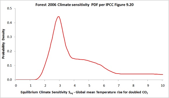
Only F06 had a climate sensitivity PDF which had its mode (peak) significantly above 2°C, leaving aside one peculiar PDF with six peaks. I found the F06 PDF’s mode of 2.9°C surprisingly high, its extended ‘shoulder’ (flattish elevated section) from 4–6°C very odd, and its failure to decline at very high sensitivity levels unsound. So, I decided back in 2011 to investigate. I should add that my main concern with F06 lay with improving the uniform-priors based Bayesian inference methodology that it shares with various other studies, which I consider greatly fattens the high climate sensitivity tail risk. The existence of two conflicting datasets was somewhat of a distraction from this concern, but an important one.
My June post largely consisted of an open letter to the chief editor of Geophysical Review Letters (GRL), in which the F06 study was published. In that letter I:
a) explained that statistical analysis suggested that the SFZ08 surface diagnostic model data was delayed by several years relative to the CSF05 data, and argued that since F06 appeared to indicate that the MIT 2D model runs extended only to 1995, on that basis the SFZ08 data could not match the timing of the observational data, which it was stated also ran to1995;
b) pointed out the surprising failure of the key surface diagnostic to provide any constraint on high climate sensitivity when using the SFZ08 data, except when ocean diffusivity was low; and
c) asked that GRL require Dr Forest to provide the processed data used in F06, the raw MIT model data having been lost, and all computer code and ancillary data used to generate the processed data and the likelihood functions from which the final results in F06 were derived.
Whilst I failed to persuade GRL to take any action, Dr Forest had a change of heart – perhaps prompted by the negative publicity at Climate Etc – and a month or so later archived what appears to be complete code used for generation of the F06 results from semi-processed data, along with the corresponding semi-processed MIT model, observational and Atmosphere-Ocean General Circulation Model (AOGCM) control run data – this last being used to estimate natural, internal variability in the diagnostic variables. I would like to thank Dr Forest for providing that data and code, and also for subsequently doing likewise for the Forest et al (2008) and Libardoni and Forest (2011) studies. I haven’t yet properly investigated the data for the 2008 and 2011 studies.
The F06 code indicated that the MIT model runs in fact extended to 2001, despite the impression I had gained from F06 that they only extended to 1995, so the argument in a) above lost its force. Compared with a diagnostic period ending in 1995, the six year difference between the SFZ08 and CSF05 surface model data could equally be due to the CSF05 data running to 2001 rather than to the SFZ08 data ending in 1989. And, indeed, that turned out to be the case. However, the data and code also indicated that the observational surface temperature data used ran to 1996, not to 1995 as stated in F06. Detailed examination and testing of the data and code confirmed that the SFZ08 surface and upper air data is the same as that used in F06, as I had thought, and that there is a timing mismatch between the model-simulated data used in SFZ08/F06, ending in 1995, and the observational data. Information helpfully provided by Dr Forest as to the model data year-end showed that the observational surface temperature data was advanced 9 months from the SFZ08/F06 model-simulated data. The CSF05 surface data has a more serious mismatch, with the model data being 63 months in advance of the observational data; it was also processed somewhat differently.
So, in summary, F06 and SFZ08 did use misprocessed data for the surface diagnostic. However, the CSF05 surface diagnostic data was substantially more flawed. Further examination of the archived code revealed some serious statistical errors in the derivation of the Forest 2006 likelihood functions. I wrote a detailed article about these errors at Climate Audit, here. But it appears that even in combination with the surface diagnostic 9 month timing mismatch these statistical errors change the F06 results only modestly.
So, why did F06 produce an estimated PDF for climate sensitivity which peaks quite sharply at a rather high Seq value, and then exhibits a strange shoulder and a non-declining tail? The answer is complex, and only the extended shoulder seems to be related to problems with the data itself. To keep this article to a reasonable length, I’m just going to deal here with remaining data issues, not other aspects of F06.
I touched on differences between the SFZ08 and the CSF05 upper air model data in my letter to GRL. In regard to the SFZ08 data (identical to that used in F06), there seems to have been some misprocessing of the 0–5°S latitude band data at most pressure levels. Data for the top (50 hPa) and bottom (850 hPa) levels is not used in this latitude band; maybe that has something to do with the problem. The chart below shows how the processed model temperature changes over the diagnostic period vary with latitude. The plot is for the best-fit Seq , Kv and Faer settings, but varies little in shape at other model parameter settings.
The latitudinal relationship varies with pressure level, as expected, but all except the 150 hPa level show values for the 0–5°S latitude band (centred at latitude -2.5) that are anomalous relative to those for adjacent bands, dipping towards zero (or, for the negative 100 hPa values, spiking up to zero).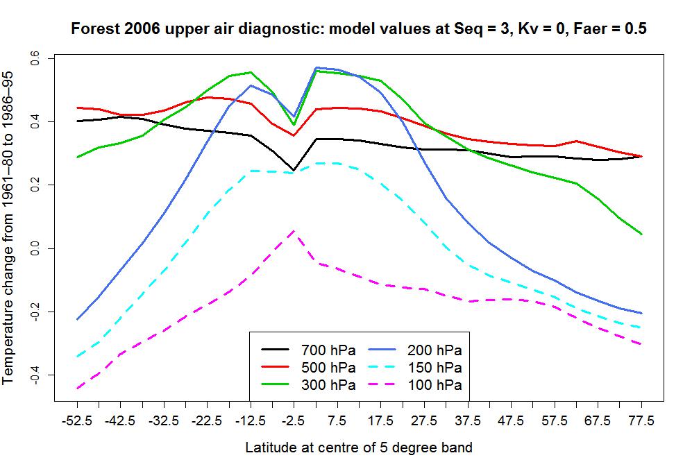
These discrepancies from adjacent values are not present in the 0–5°S band model data at an earlier stage of processing. I haven’t been able to work out what causes them. The observations are too noisy to tell much from, but they don’t show similar dips for the 0–5°S latitude band.
So, what effect do these suspicious-looking 0–5°S latitude band model-simulated upper air values have? In practice, the effects of even major resulting changes in the upper air diagnostic likelihood function values are not that dramatic, since the surface diagnostic provides more powerful inference and, along with the deep ocean diagnostic, dominates the final parameter PDFs. But the effects of the upper air diagnostic are not negligible. I show below a plot of estimated climate sensitivity PDFs for F06, all based on uniform priors and the same stated method, based on different ways of treating the upper air data. Before interpreting it, I need to explain a couple of things.
Interpolation
It is necessary to interpolate from values at the 460 odd model-run locations to a regular fine 3D grid, with over 300,000 locations, spanning the range of Seq, Kv and Faer values. In F06, the sum-of-squares, r2, of the differences between model-simulated and observed temperature changes was interpolated – one variable for each grid location. I instead independently interpolated the circa 220 model-simulated values, and calculated r2 values using those smoothed values. That makes it feasible, by forcing the interpolated surfaces to be smoother, to allow for model noise (internal variability). The fine grid r2 values are used to calculate the likelihood of the corresponding Seq, Kv and Faer combination being correct, and hence (when combined with likelihoods from the other diagnostics, and multiplied by the chosen prior distributions) to derive estimated PDFs for each of Seq, Kv and Faer.
Truncation parameter
The truncation parameter, k, affects how much detail is retained when calculating the r2 values. The higher the truncation parameter, the better is discrimination between differing values of Seq, Kv and Faer. However, if k is too high then the r2 values will be heavily affected by noise and be unreliable. F06 used k = 14. I reckon k = 12 gives more reliable results.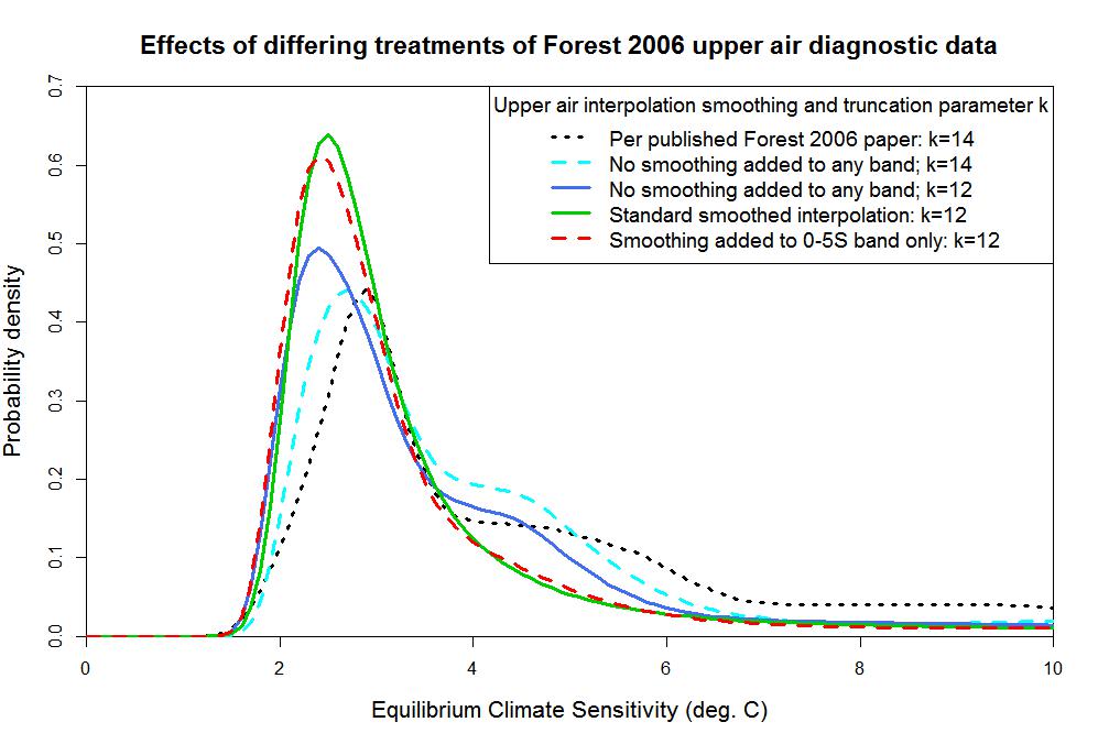
Now I’ll work through the PDF curves, in the same order as in the legend:
The dotted black line is the F06 PDF as originally published in GRL (as per the red line in the first graph).
The dashed cyan line shows my estimated PDF without adding any interpolation smoothing, using the same truncation parameter, k = 14, as in F06. A shoulder on the upper side of the peak is clearly present between Seq = 4°C and Seq = 5°C, although this does not extend as far as the one in the original F06 PDF. Also, the peak of the PDF (the mode) is slightly lower, at 2.7°C rather than 2.9°C, and at very high Seq the PDF curve flattens out at a lower value than does the F06 one. The differences probably arise both from the differences in interpolation method and from F06 having mis-implemented its method in several ways. As well as the statistical errors already mentioned, F06’s calculation of the upper air diagnostic r2 values was wrong.
The solid blue line is on the same basis as the dashed cyan line except that I have reduced the truncation parameter k from 14 to 12. Doing so modestly reduces the mode of the PDF, to 2.4°C, and lowers the height of the shoulder (resulting in the peak height of the PDF increasing slightly).
The solid green line is on the same basis as the solid blue line except that I have used my standard interpolation basis, adding sufficient smoothing (the same for all latitude bands and pressure levels) to allow for model noise. The effect is very noticeable: the shoulder on the RHS completely disappears, giving a more normal shape to the PDF. The mode and the extreme upper tail are little changed.
Remember that model data for each latitude band and pressure level is interpolated separately, so interpolation smoothing does not result in incorrect values in the 0–5°S latitude band being adjusted by reference to values in the adjacent bands. However, some people may nevertheless be suspicious about making the interpolation smoother.
Now look at the dashed red line. Here, I have melded the interpolated data used to produce the solid blue and green curves, only using the added smoothing (green line) version for the 0–5°S latitude band – 6 out of some 220 diagnostic variables. Yet the resulting PDF is almost identical to the green line. That is powerful evidence for concluding that the shoulder in the F06 PDF is caused by misprocessing of the 0–5°S latitude band upper air model-simulation data. The probable explanation is that misprocessed values are insufficiently erroneous to seriously affect the r2 values except where model noise adds to the misprocessing error, and that the interpolation method I use is, with added smoothing, very effective at removing model noise.
Although not shown, I have also computed PDFs either excluding the 0–5°S latitude band data entirely, or replacing it with a second copy of the 0–5°N latitude band data: there should be little latitudinal variation of upper air temperatures in the inner tropics. In both cases, the resulting PDF is very similar to the green and dashed red lines. That very much confirms my conclusion.
So, to conclude regarding data issues, both the surface and upper air F06 data had been misprocessed, although only in the case of the upper air data was the processing so badly flawed that there was an appreciable effect on the estimated climate sensitivity PDF. This case provides a useful illustration of the importance of archiving computer code as well as data – without both being available, none of the errors in F06’s processing of its data would have come to light.
Nicholas Lewis
Leave A Comment