Originally a guest post on April 16, 2013 at Watts Up With That?
Many readers will know that I have analysed the Forest et al., 2006, (F06) study in some depth. I’m pleased to report that my paper reanalysing F06 using an improved, objective Bayesian method was accepted by Journal of Climate last month, just before the IPCC deadline for papers to be cited in AR5 WG1, and has now been posted as an Early Online Release, here. The paper is long (8,400 words) and technical, with quite a lot of statistical mathematics, so in this article I’ll just give a flavour of it and summarize its results.
The journey from initially looking into F06 to getting my paper accepted was fairly long and bumpy. I originally submitted the paper last July, fourteen months after first coming across some data that should have matched what was used in F06. The reason it took me that long was partly that I was feeling my way, learning exactly how F06 worked, how to undertake objective statistical inference correctly in its case and how to deal with other issues that I was unfamiliar with. It was also partly because after some months I obtained, from the lead author of a related study, another set of data that should have matched the data used in F06, but which was mostly different from the first set. And it was partly because I was unsuccessful in my attempts to obtain any data or code from Dr Forest.
Fortunately, he released a full set of (semi-processed) data and code after I submitted the paper. Therefore, in a revised version of the paper submitted in December, following a first round of peer review, I was able properly to resolve the data issues and also to take advantage of the final six years of model simulation data, which had not been used in F06. I still faced difficulties with two reviewers – my response to one second review exceeded 9,500 words – but fortunately the editor involved was very fair and helpful, and decided my re-revised paper did not require a further round of peer review.
Forest 2006
First, some details about F06, for those interested. F06 was a ‘Bayesian’ study that estimated climate sensitivity (ECS or Seq) jointly with effective ocean diffusivity (Kv)1 and aerosol forcing (Faer). F06 used three ‘diagnostics’ (groups of variables whose observed values are compared to model-simulations): surface temperature anomalies, global deep-ocean temperature trend, and upper-air temperature changes. The MIT 2D climate model, which has adjustable parameters calibrated in terms of Seq , Kv and Faer, was run several hundred times at different settings of those parameters, producing sets of model-simulated temperature changes. Comparison of these simulated temperature changes to observations provided estimates of how likely the observations were to have occurred at each set of parameter values (taking account of natural internal variability). Bayes’ theorem could then be applied, uniform prior distributions for the three parameters being multiplied together, and the resulting uniform joint prior being multiplied by the likelihood function for each diagnostic in turn. The result was a joint posterior probability density function (PDF) for the parameters. The PDFs for each of the individual parameters were then readily derived by integration. These techniques are described in Appendix 9.B of AR4 WG1, here.
Lewis 2013
As noted above, Forest 06 used uniform priors in the parameters. However, the relationship between the parameters and the observations is highly nonlinear and the use of a uniform parameter prior therefore strongly influences the final PDF. Therefore in my paper Bayes’ theorem is applied to the data rather than the parameters: a joint posterior PDF for the observations is obtained from a joint uniform prior in the observations and the likelihood functions. Because the observations have first been ‘whitened’,2 this uniform prior is noninformative, meaning that the joint posterior PDF is objective and free of bias. Then, using a standard statistical formula, this posterior PDF in the whitened observations can be converted to an objective joint PDF for the climate parameters.
The F06 ECS PDF had a mode (most likely value) of 2.9 K (°C) and a 5–95% uncertainty range of 2.1 to 8.9 K. Using the same data, I estimate a climate sensitivity PDF with a mode of 2.4 K and a 5–95% uncertainty range of 2.0–3.6 K, the reduction being primarily due to use of an objective Bayesian approach. Upon incorporating six additional years of model-simulation data, previously unused, and improving diagnostic power by changing how the surface temperature data is used, the central estimate of climate sensitivity using the objective Bayesian method falls to 1.6 K (mode and median), with 5–95% bounds of 1.2–2.2 K. When uncertainties in non-aerosol forcings and in surface temperatures, ignored in F06, are allowed for, the 5–95% range widens to 1.0–3.0 K.
The 1.6 K mode for climate sensitivity I obtain is identical to the modes from Aldrin et al. (2012) and (using the same, HadCRUT4, observational dataset) Ring et al. (2012). It is also the same as the best estimate I obtained in my December non-peer reviewed heat balance (energy budget) study using more recent data, here. In principle, the lack of warming over the last ten to fifteen years shouldn’t really affect estimates of climate sensitivity, as a lower global surface temperature should be compensated for by more heat going into the ocean.
Footnotes
- Parameterised as its square root
- Making them uncorrelated, with a radially symmetric joint probability density
The below plot shows how the factor for converting the joint PDF for the whitened observations into a joint PDF for the three climate system parameters (on the vertical axis – units arbitrary) varies with climate sensitivity Seq and ocean diffusivity Kv. This conversion factor is, mathematically, equivalent to a noninformative joint prior for the parameters. The plot is for a slightly different case to that illustrated in the paper, but its shape is almost identical. Aerosol forcing has been set to a fixed value. At different aerosol values the surface scales up or down somewhat, but retains its overall shape.
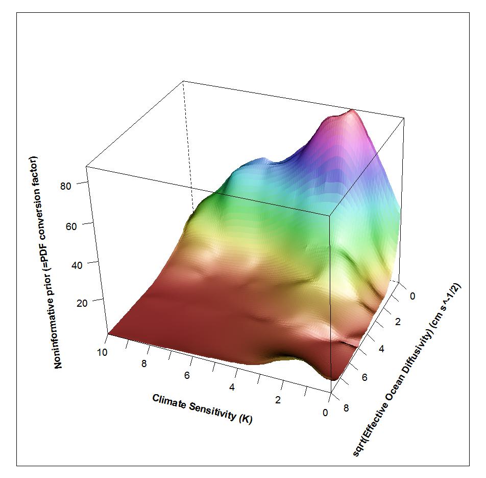
The key thing to notice is that at high sensitivity values not only does the prior tail off even when ocean diffusivity is low, but that at higher Kv values the prior becomes almost zero. (Ignore the upturn in the front RH corner, which is caused by model noise.) The noninformative prior thereby prevents more probability than the data uncertainty distributions warrant being assigned to regions where data responds little to parameter changes. It is that which results in better-constrained PDFs being, correctly, obtained compared to when uniform priors for the parameters are used.
Leave A Comment