Originally a guest post on Apr 17, 2014 – 10:04 AM at Climate Audit
On 1 April 2014 the Bishop Hill blog carried a guest post ‘Dating error’ by Doug Keenan, in which he set out his allegations of research misconduct by Oxford University professor Christopher Bronk Ramsey. Professor Bronk Ramsey is an expert on calibration of radiocarbon dating and author of OxCal, apparently one of the two most widely used radiocarbon calibration programs (the other being Calib, by Stuiver and Reimer). Steve McIntyre and others opined that an allegation of misconduct was inappropriate in this sort of case, and likely to be counter-productive. I entirely agree. Nevertheless, the post prompted an interesting discussion with statistical expert Professor Radford Neal of Toronto University and with Nullius in Verba (an anonymous but statistically-minded commentator). They took issue with Doug’s claims that the statistical methods and resulting probability densities (PDFs) and probability ranges given by OxCal and Calib are wrong. Doug’s arguments, using a partly Bayesian approach he calls a discrete calibration method, are set out in his 2012 peer reviewed paper.
I also commented, saying if one assumes a uniform prior for the true calendar date, then Doug Keenan’s results do not follow from standard Bayesian theory. Although the OxCal and Calib calibration graphs (and the Calib manual) are confusing on the point, Bronk Ramsey’s papers make clear he does use such a uniform prior. I wrote that in my view Bronk Ramsey had followed a defensible approach (since his results flow from applying Bayes’ theorem using that prior), so there was no research misconduct involved, but that his method did not represent best scientific inference.
The final outcome was that Doug accepted what Radford and Nullius said about how the sample measurement should be interpreted as probability, with the implication that his criticism of the calibration method is invalid. However, as I had told Doug originally, I think his criticism of the OxCal and Calib calibration methods is actually valid: I just think that imperfect understanding rather than misconduct on the part of Bronk Ramsey (and of other radiocarbon calibration experts) is involved. Progress in probability and statistics has for a long time been impeded by quasi-philosophical disagreements between theoreticians as to what probability represents and the correct foundations for statistics. Use of what are, in my view, unsatisfactory methods remains common.
Fortunately, regardless of foundational disagreements I think most people (and certainly most scientists) are in practice prepared to judge the appropriateness of statistical estimation methods by how well they perform upon repeated use. In other words, when estimating the value of a fixed but unknown parameter, does the true value lie outside the specified uncertainty range in the indicated proportion of cases?
This so-called frequentist coverage or probability-matching property can be tested by drawing samples at random from the relevant uncertainty distributions. For any assumed distribution of parameter values, a method of producing 5–95% uncertainty ranges can be tested by drawing a large number of samples of possible parameter values from that distribution, and for each drawing a measurement at random according to the measurement uncertainty distribution and estimating a range for the parameter. If the true value of the parameter lies below the bottom end of the range in 5% of cases and above its top in 5% of cases, then that method can be said to exhibit perfect frequentist coverage or exact probability matching (at least at the 5% and 95% probability levels), and would be viewed as a more reliable method than a non-probability-matching one for which those percentages were (say) 3% and 10%. It is also preferable to a method for which those percentages were both 3%, which would imply the uncertainty ranges were unnecessarily wide. Note that in some cases probability-matching accuracy is unaffected by the parameter value distribution assumed.
I’ll now attempt to explain the statistical issues and to provide evidence for my views. I’ll then set up a simplified, analytically tractable, version of the problem and use it to test the probability matching performance of different methods. I’ll leave discussion of the merits of Doug’s methods to the end.
2. Statistical issues involved in radiocarbon calibration
The key point is that OxCal and Calib use a subjective Bayesian method with a wide uniform prior on the parameter being estimated, here calendar age, whilst the observational data provides information about a variable, radiocarbon or 14C age, that has a nonlinear relationship to the parameter of interest. The vast bulk of the uncertainty relates to 14C age – principally measurement and similar errors, but also calibration uncertainty. The situation is thus very similar to that for estimation of climate sensitivity. It seems to me that the OxCal and Calib methods are conceptually wrong, just as use of a uniform prior for estimating climate sensitivity is normally inappropriate.
In the case of climate sensitivity, I have been arguing for a long time that Bayesian methods are only appropriate if one takes an objective approach, using a noninformative prior, rather than a subjective approach (using, typically, a uniform or expert prior). Unfortunately, many statisticians (and all but a few climate scientists) seem not to understand, or at least not to accept, the arguments in favour of an objective Bayesian approach. Most climate sensitivity studies still use subjective Bayesian methods.
Objective Bayesian methods require a noninformative prior. That is, a prior that influences parameter estimation as little as possible: it lets the data ‘speak for themselves’[i]. Bayesian methods generally cannot achieve exact probability matching even with the most noninformative prior, but objective Bayesian methods can often achieve approximate probability matching. In simple cases a uniform prior is quite often noninformative, so that a subjective Bayesian approach that involved using a uniform prior would involve the same calculations and give the same results as an objective Bayesian approach. An example is where the parameter being estimated is linearly related to data, the uncertainties in which represent measurement errors with a fixed distribution. However, where nonlinear relationships are involved a noninformative prior for the parameter is rarely uniform. In complex cases deriving a suitable noninformative prior can be difficult, and in many cases it is impossible to find a prior that has no influence at all on parameter estimation.
Fortunately, in one-dimensional cases where uncertainty involves measurement and similar errors it is often possible to find a completely noninformative prior, with the result that exact probability matching can be achieved. In such cases, the so-called ‘Jeffreys’ prior’ is generally the correct choice, and can be calculated by applying standard formulae. In essence, Jeffreys’ prior can be thought of as a conversion factor between distances in parameter space and distances in data space. Where a data–parameter relationship is linear and the data error distribution is independent of the parameter value, that conversion factor will be fixed, leading to Jeffreys’ prior being uniform. But where a data–parameter relationship is nonlinear and/or the data precision is variable, Jeffreys’ prior achieves noninformativeness by being appropriately non-uniform.
Turning to the specifics of radiocarbon dating, my understanding is as follows. The 14C age uncertainty varies with 14C age, and is lognormal rather than normal (Gaussian). However, the variation in uncertainty is sufficiently slow for the error distribution applying to any particular sample to be taken as Gaussian with a standard deviation that is constant over the width of the distribution, provided the measurement is not close to the background radiation level. It follows that, were one simply estimating the ‘true’ radiocarbon age of the sample, a uniform-in-14C-age prior would be noninformative. Use of such a prior would result in an objective Bayesian estimated posterior PDF for the true 14C age that was Gaussian in form.
However, the key point about radiocarbon dating is that the ‘calibration curve’ relationship of ‘true’ radiocarbon age t14C to the true calendar date ti of the event corresponding to the 14C determination is highly nonlinear. (I will consider only a single event, so i = 1.) It follows that to be noninformative a prior for ti must be non-uniform. Assuming that the desire is to produce uncertainty ranges beyond which – upon repeated use – the true calendar date will fall in a specified proportion of cases, the fact that in reality there may be an equal chance of tilying in any calendar year is irrelevant.
The Bayesian statistical basis underlying the OxCal method is set out in a 2009 paper by Bronk Ramsey[ii]. I will only consider the simple case of a single event, with all information coming from a single 14C determination. Bronk Ramsey’s paper states:
The likelihood defines the probability of obtaining a measurement given a particular date for an event. If we only have a single event, we normally take the prior for the date of the event to be uniform (but unnormalized):
p(ti) ~ U(–∞,∞ ) ~ constant
Defensible though it is in terms of subjective Bayesian theory, a uniform prior in titranslates into a highly non-uniform prior for the ‘true’ radiocarbon age (t14C) as inferred from the 14C determination. Applying Bayes’ theorem in the usual way, the posterior density for t14C will then be non-Gaussian.
The position is actually more complicated, in that the calibration curve itself also has uncertainty, which is also assumed to be Gaussian in form. One can think of there being a nonlinear but exact functional calibration curve relationship s14C = c(ti) between calendar year ti and a ‘standard’ 14C age s14C, but with – for each calendar year – the actual (true, not measured) 14C age t14C having a slightly indeterminate relationship with ti. So the statistical relationship (N signifying a normal or Gaussian distribution having the stated mean and standard deviation ) is:
t14C ~ N(c(ti), σc(ti)) (1)
where σc is the calibration uncertainty standard deviation, which in general will be a function of ti. In turn, the radiocarbon determination age d14C is assumed to have the form
d14C ~ N(t14C, σd) (2)
with the variation of the standard deviation σd with t14C usually being ignored for individual samples.
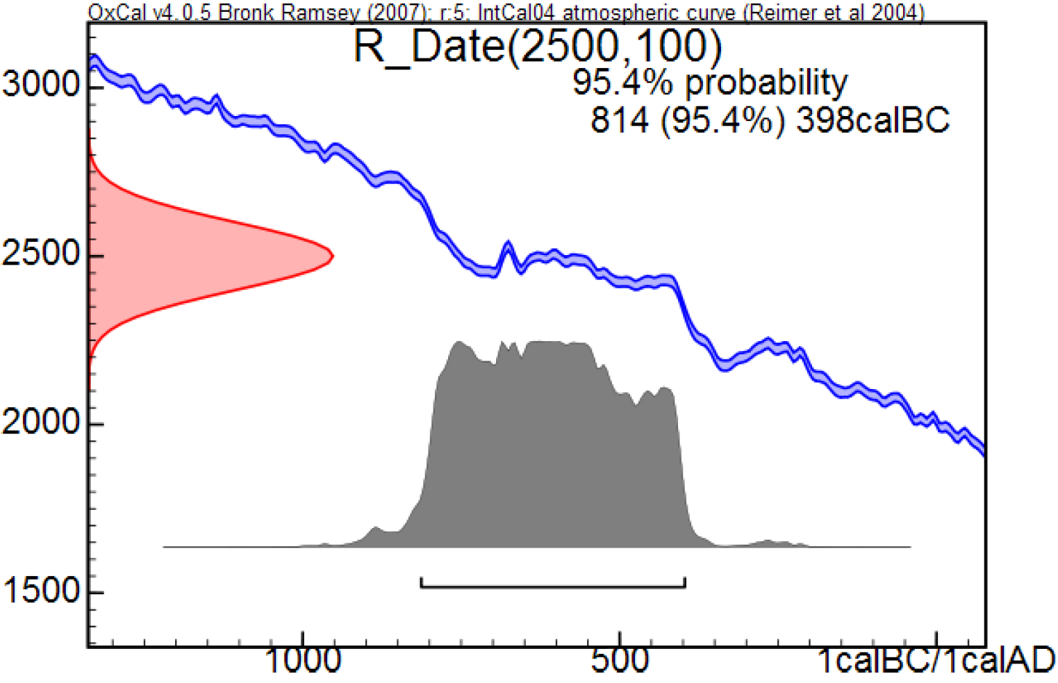
Fig. 1: Example OxCal calibration (from Fig.1 of Keenan, 2012, Calibration of a radiocarbon age)
Figure 1, from Fig. 1 in Doug’s paper, shows an example of an OxCal calibration, with the resulting 95.4% (±2 sigma for a Gaussian distribution) probability range marked by the thin bar above the x-axis. The red curve on the y-axis is centred on the 14C age derived by measurement (the radiocarbon or 14C determination) and shows the likelihood for that determination as a function of true 14C age. The likelihood for a 14C determination is the relative probability, for any given true 14C age, of having obtained that determination given the uncertainty in 14C determinations. The blue calibration curve shows the relationship between true 14C age (on the y-axis) and true calendar age on the x-axis. Its vertical width represents calibration uncertainty. The estimated PDF for calendar age is shown in grey. Ignoring the small effect of the calibration uncertainty, the PDF simply expresses the 14C determination’s likelihood as a function of calendar age. It represents both the likelihood function for the determination and – since a uniform prior for calendar age is used – the posterior PDF for the true calendar age (Bayes’ theorem giving the posterior as the normalised product of the prior and the likelihood function).
By contrast to OxCal’s subjective Bayesian, uniform prior based method, an objective Bayesian approach would involve computing a noninformative prior for ti. The standard choice would normally be Jeffreys’ prior. Doing so is somewhat problematic here in view of the calibration curve not being monotonic – it contains reversals – and also having varying uncertainty.
If the calibration curve were monotonic and had an unvarying error magnitude, the calibration curve error could be absorbed into a slightly increased 14C determination error, as both these uncertainty distributions are assumed Gaussian. Since the calibration curve error appears small in relation to 14C determination error, and typically only modestly varying over the 14C determination error range, I will make the simplifying assumption that it can be absorbed into an increased 14C determination error. The statistical relationship then becomes, given independence of calibration curve and radiocarbon determination uncertainty:
d14C ~ N( c(ti), sqrt(σc²+σd²) ) (3)
On that basis, and ignoring also the calibration curve being limited in range, it follows that Jeffreys’ prior for ti would equal the absolute derivative (slope) of calibrated 14C age with respect to calendar date. Moreover, in the absence of non-monotonicity it is known that in a case like this the Jeffreys’ prior is completely noninformative. Jeffreys’ prior would in fact provide exact probability matching – perfect agreement between the objective Bayesian posterior cumulative distribution functions (CDFs – the integrals of PDFs) and the results of repeated testing. The reason for the form here of Jeffreys’ prior is fairly clear – where the calibration curve is steep and hence its derivative with respect to calendar age is large, the error probability (red shaded area) between two nearby values of t14C corresponds to a much smaller ti range than when the derivative is small.
An alternative way of seeing that a noninformative prior for calendar age should be proportional to the derivative of the calibration curve is as follows. One can perform the Bayesian inference step to derive a posterior PDF for the true 14C age, t14C, using a uniform prior for 14C age – which as stated previously is, given the assumed Gaussian error distribution, noninformative. That results in a posterior PDF for 14C age that is identical, up to proportionality, to its likelihood function. Then one can carry out a change of variable from t14C to ti. The standard (Jacobian determinant) formula for converting a PDF between two variables, where one is a function of the other, involves multiplying the PDF, expressed in terms of the new variable, by the absolute derivative of the inverse transformation – the derivative of t14C with respect to ti. Taking this route, the objective posterior PDF for calendar age is the normalised product of the 14C age likelihood function (since the 14C objective Bayesian posterior is proportional to its likelihood function), expressed in terms of calendar age, multiplied by the derivative of t14C with respect to ti. That is identical, as it should be, to the result of direct objective Bayesian inference of calendar age using the Jeffreys’ prior.
3. Examining various methods using a simple stylised calibration curve
In order to make the problem analytically tractable and the performance of different methods – in terms of probability matching – easily testable, I have created a stylised calibration curve. It consists of the sum of three scaled shifted sigmoid functions. The curve exhibits both plateaus and steep regions whilst being smooth and monotonic and having a simple derivative.
Figure 2 shows similar information to Figure 1 but with my stylised calibration curve instead of a real one. The grey wings of the curve represent a fixed calibration curve error, which, as discussed, I absorb into the 14C determination error. The pink curve, showing the Bayesian posterior PDF using a uniform prior in calendar age, corresponds to the grey curve in Figure 1. It is highest over the right hand plateau, which corresponds to the centre of the red radiocarbon age error distribution, but has a non-negligible value over the left hand plateau as well. The figure also shows the objective Jeffreys’ prior (dotted green line), which reflects the derivative of the calibration curve. The objective Bayesian posterior using that prior is shown as the solid green line. As can be seen, it is very different from the uniform-calendar-year-prior based posterior that would be produced by the OxCal or Calib programs for this 14C determination (if they used this calibration curve).
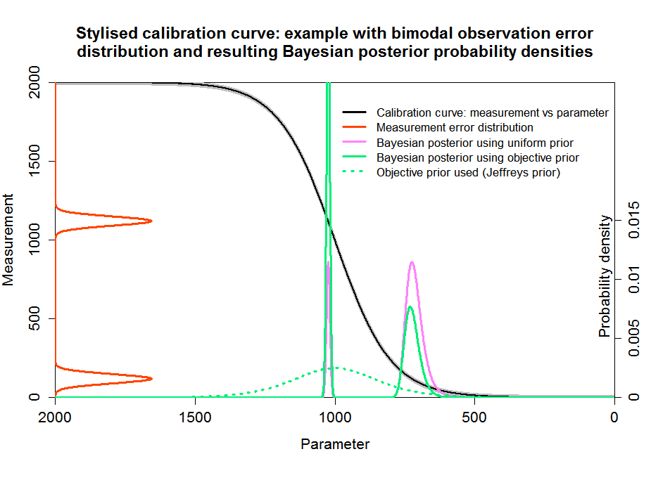
The Jeffreys’ prior (dotted green line) has bumps wherever the calibration curve has a high slope, and is very low in plateau regions. Subjective Bayesians will probably throw up their hands in horror at it, since it would be unphysical to think that the probability of a sample having any particular calendar age depended on the shape of the calibration curve. But that is to mistake the nature of a noninformative prior, here Jeffreys’ prior. A noninformative prior has no direct probabilistic interpretation. As a standard textbook (Bernardo and Smith, 1994) puts it in relation to reference analysis, arguably the most successful approach to objective Bayesian inference: “The positive functions π(θ) [the noninformative reference priors] are merely pragmatically convenient tools for the derivation of reference posterior distributions via Bayes’ theorem”.
Rather than representing a probabilistic description of existing evidence as to a probability distribution for the parameter being estimated, a noninformative prior primarily reflects (at least in straightforward cases) how informative, at differing values of the parameter, the data is expected to be about the parameter. That in turn reflects how precise the data are in the relevant region and how fast expected data values change with the parameter value. This comes back to the relationship between distances in parameter space and distances in data space that I mentioned earlier.
It may be thought that the objective posterior PDF has an artificial shape, with peaks and low regions determined, via the prior, by the vagaries of the calibration curve and not by genuine information as to the true calendar age of the sample. But one shouldn’t pay too much attention to PDF shapes; they can be misleading. What is most important in my view is the calendar age ranges the PDF provides, which for one-sided ranges follow directly from percentage points of the posterior CDF.
By a one-sided x% range I mean the range from the lowest possible value of the parameter (here, zero) to the value, y, at which the range is stated to contain x% of the posterior probability. An x1–x2% range or interval for the parameter is then y1 − y2, where y1 and y2 are the (tops of the) one-sided x1% and x2% ranges. Technically, this is a credible interval, as it relates to Bayesian posterior probability.
By contrast, a (frequentist) x% one-sided confidence interval with a limit of y can, if accurate, be thought of as one calculated to result in values of y such that, upon indefinitely repeated random sampling from the uncertainty distributions involved, the true parameter value will lie below y in x% of cases. By definition, an accurate confidence interval exhibits perfect frequentist coverage and so represents, for an x% interval, exact probability matching. If one-sided Bayesian credible intervals derived using a particular prior pass that test then they and the prior used are said to be probability matching. In general, Bayesian posteriors cannot be perfectly probability matching. But the simplified case presented here falls within an exception to that rule, and use of Jeffreys’ prior should in principle lead to exact probability matching.
The two posterior PDFs in Figure 2 imply very different calendar age uncertainty ranges. As OxCal reports a 95.4% range, I’ll start with the 95.4% ranges lying between the 2.3% and 97.7% points of each posterior CDF. Using a uniform prior, that range is 365–1567 years. Using Jeffreys’ prior, the objective Bayesian 2.3–97.7% range is 320–1636 years – somewhat wider. But for a 5–95% range, the difference is large: 395–1472 years using a uniform prior versus 333–1043 years using Jeffreys’ prior.
Note that OxCal would report a 95.4% highest posterior density (HPD) range rather than a range lying between the 2.3% and 97.7% points the posterior CDF. A 95.4% HPD range is one spanning the region with the highest posterior densities that includes 0.954 probability in total; it is necessarily the narrowest such range. HPD ranges are located differently from those with equal probability in both tails of a probability distribution; they are narrower but not necessarily better.
What about confidence intervals, a non-Bayesian statistician would rightly ask? The obvious way of obtaining confidence intervals is to use likelihood-based inference, specifically the signed root log-likelihood ratio (SRLR). In general, the SRLR only provides approximate confidence intervals. But where, as here, the parameter involved is a monotonic transform of a variable with a Gaussian distribution, SRLR confidence intervals are exact. So what are the 2.3–97.7% and 5–95% SRLR-derived confidence intervals? They are respectively 320–1636 years and 333–1043 years – identical to the objective Bayesian ranges using Jeffreys’ prior, but quite different from those using a uniform prior. I would argue that the coincidence of the Jeffreys’ prior derived objective Bayesian credible intervals and the SRLR confidence intervals reflects the fact that here both methods provide exact probability matching.
4. Numerical testing of different methods using the stylised calibration curve
Whilst an example is illuminating, in order properly to compare the performance of the different methods one needs to carry out repeated testing of probability matching based on a large number of samples: frequentist coverage testing. Although some Bayesians reject such testing, most people (including most statisticians) want a statistical inference method to produce, over the long run, results that accord with relative frequencies of outcomes from repeated tests involving random draws from the relevant probability distributions. By drawing samples from the same uniform calendar age distribution on which Bronk Ramsey’s method is predicated, we can test how well each method meets that aim. This is a standard way of testing statistical inference methods. Clearly, one wants a method also to produce accurate results for samples that – unbeknownst to the experimenter – are drawn from individual regions of the age range, and not just for samples that have an equal probability of having come from any year throughout the entire range.
I have accordingly carried out frequentist coverage testing, using 10,000 samples drawn at random uniformly from both the full extent of my calibration curve and from various sub-regions of it. For each sampled true calendar age, a 14C determination age is sampled randomly from a Gaussian error distribution. I’ve assumed an error standard deviation of 30 14C years, to include calibration curve uncertainty as well as that in the 14C determination. Whilst in principle I should have used somewhat different illustrative standard deviations for different regions, doing so would not affect the qualitative findings.
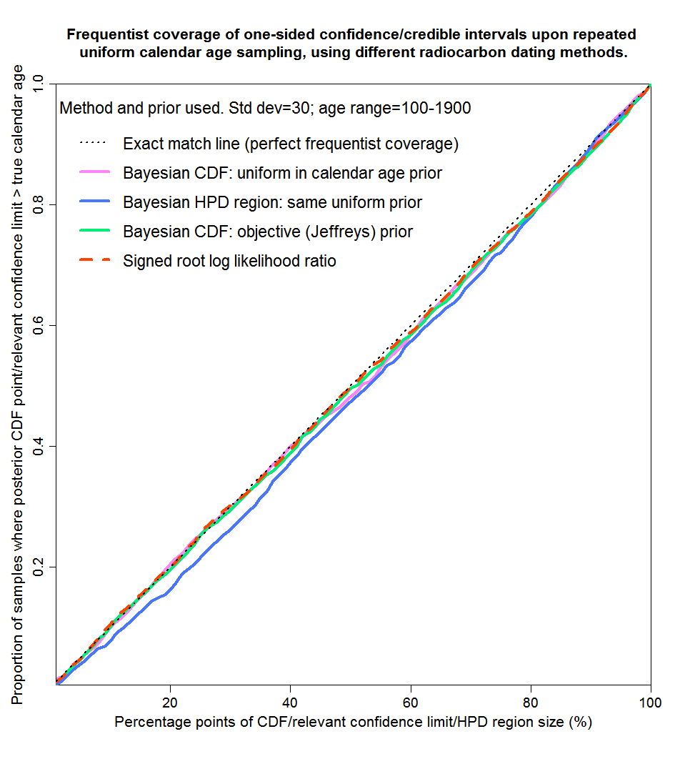
In these frequentist coverage tests, for each integral percentage point of probability the proportion of cases where the true calendar age of the sample falls below the upper limit given by the method involved for a one-sided interval extending to that percentage point is computed. The resulting proportions are then plotted against the percentage points they relate to. Perfect probability matching will result in a straight line going from (0%, 0) to (100%,1). I test both subjective and objective Bayesian methods, using for calendar age respectively a uniform prior and Jeffreys’ prior. I also test the signed root log-likelihood ratio method.
For the Bayesian method using a uniform prior, I also test the coverage of the HPD regions that OxCal reports. As HPD regions are two-sided, I compute the proportion of cases in which the true calendar age falls within the calculated HPD region for each integral percentage HPD region. Since usually only ranges that contain a majority of the estimated posterior probability are of interest, only the right hand half of the HPD curves (HPD ranges exceeding 50%) is of practical significance. Note that the title and y-axis label in the frequentist coverage test figures refer to one-sided regions and should in relation to HPD regions be interpreted in accordance with the foregoing explanation.
I’ll start with the entire range, except that I don’t sample from the 100 years at each end of the calibration curve. That is because otherwise a significant proportion of samples result in non-negligible likelihood falling outside the limits of the calibration curve. Figure 3 accordingly shows probability matching with true calendar ages drawn uniformly from years 100–1900. The results are shown for four methods. The first two are subjective Bayesian using a uniform prior as per Bronk Ramsey – from percentage points of the posterior CDF and from highest posterior density regions. The third is objective Bayesian employing Jeffreys’ prior, from percentage points of the posterior CDF. The fourth uses the non-Bayesian signed root log-likelihood ratio (SRLR) method. In this case, all four methods give good probability matching – their curves lie very close to the dotted black straight line that represents perfect matching.
Now let’s look at sub-periods of the full 100–1900 year period. I’ve picked periods representing both ranges over which the calibration curve is mainly flattish and those where it is mainly steep. I start with years 100–500, over most of which the calibration curve is steep. The results are shown in Figure 4. Over this period, SRLR gives essentially perfect matching, while the Bayesian methods give mixed results. Jeffreys’ prior gives very good matching – not quite perfect, probably because for some samples there is non-negligible likelihood at year zero. However, posterior CDF points using a uniform prior don’t provide very good matching, particularly for small values of the CDF (corresponding to the lower bound of two-sided uncertainty ranges). Posterior HPD regions provide rather better, but still noticeably imperfect, matching.
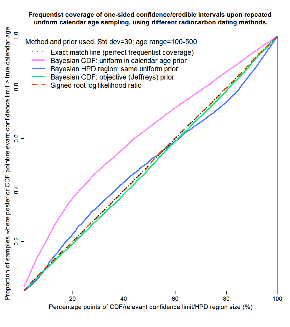
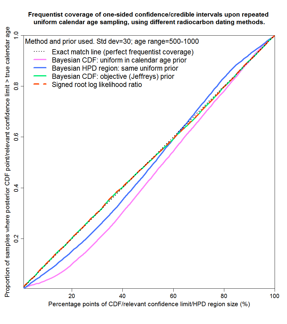
Figure 5 shows results for the 500–1000 range, which is flat except near 1000 years. The conclusions are much as for 100–500 years save that Jeffreys’ prior now gives perfect matching and that mismatching from posterior CDF points resulting from a uniform prior give smaller errors (and in the opposite direction) than for 100–500 years.
Now we’ll take the 1000–1100 years range, which asymmetrically covers a steep region in between two plateaus of the calibration curve. As Figure 6 shows, this really separates the sheep from the goats. The SRLR and objective Bayesian methods continue to provide virtually perfect probability matching. But the mismatching from the posterior CDF points resulting from a uniform prior Bayesian method is truly dreadful, as is that from HPD regions derived using that method. The true calendar age would only lie inside a reported 90% HPD region for some 75% of samples. And over 50% of samples would fall below the bottom of a 10–90% credible region given by the posterior CDF points using a uniform prior. Not a very credible region at all.
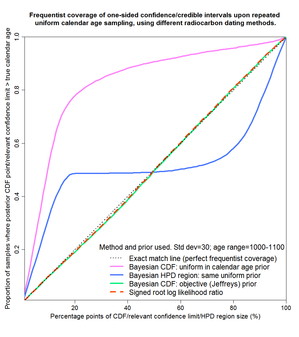
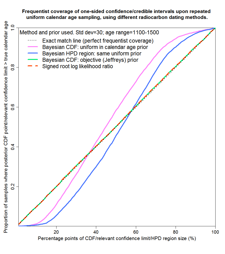
Figure 7 shows that for the next range, 1100–1500 years, where the calibration curve is largely flat, the SRLR and objective Bayesian methods again provide virtually perfect probability matching. However, the uniform prior Bayesian method again fails to provide reasonable probability matching, although not as spectacularly badly as over 1000–1100 years. In this case, symmetrical credible regions derived from posterior CDF percentage points, and HPD regions of over 50% in size, will generally contain a significantly higher proportion of the samples than the stated probability level of the region – the regions will be unnecessarily wide.
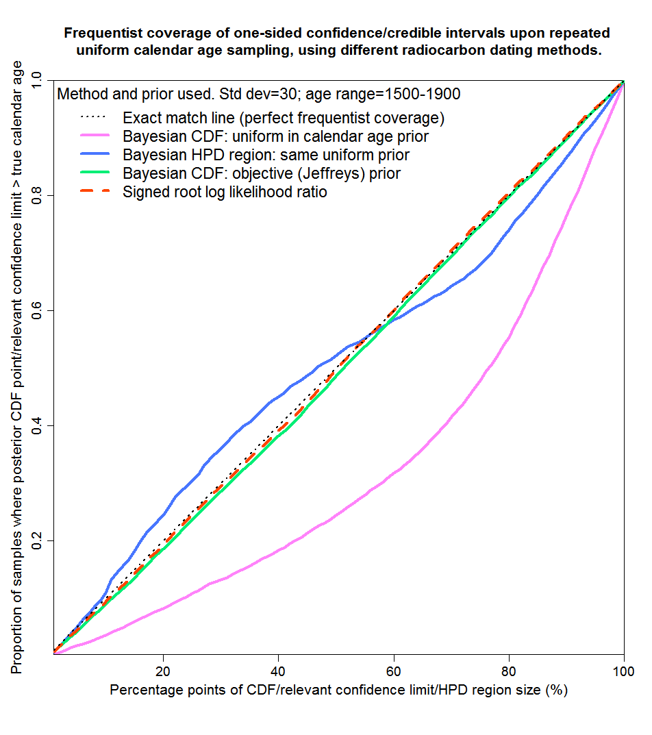
Finally, Figure 8 shows probability matching for the mainly steep 1500–1900 years range. Results are similar to those for years 100–500, although the uniform prior Bayesian method gives rather worse matching than it does for years 100–500. Using a uniform prior, the true calendar age lies outside the HPD region noticeably more often than it should, and lies beyond the top of credible regions derived from the posterior CDF twice as often as it should.
5. Discussion and Conclusions
The results of the testing are pretty clear. In whatever range the true calendar age of the sample lies, both the objective Bayesian method using a noninformative Jeffreys’ prior and the non-Bayesian SRLR method provide excellent probability matching – almost perfect frequentist coverage. Both variants of the subjective Bayesian method using a uniform prior are unreliable. The HPD regions that OxCal provides give less poor coverage than two-sided credible intervals derived from percentage points of the uniform prior posterior CDF, but at the expense of not giving any information as to how the missing probability is divided between the regions above and below the HPD region. For both variants of the uniform prior subjective Bayesian method, probability matching is nothing like exact except in the unrealistic case where the sample is drawn equally from the entire calibration range – in which case over-coverage errors in some regions on average cancel out with under-coverage errors in other regions, probably reflecting the near symmetrical form of the stylised overall calibration curve.
I have repeated the above tests using 14C error standard deviations of 10 years and 60 years instead of 30 years. Results are qualitatively the same.
Although I think my stylised calibration curve captures the essence of the principal statistical problem affecting radiocarbon calibration, unlike real 14C calibration curves it is monotonic. It also doesn’t exhibit variation of calibration error with age, but such variation shouldn’t have a significant impact unless, over the range where the likelihood function for the sample is significant, it is substantial in relation to 14C determination error. Non-monotonicity is more of an issue, and could lead to noticeable differences between inference from an objective Bayesian method using Jeffreys’ prior and from the SRLR method. If so, I think the SRLR results are probably to be preferred, where it gives a unique contiguous confidence interval. Jeffreys’ prior, which in effect converts length elements in 14C space to length elements in calendar age space, may convert single length elements in 14C space to multiple length elements in calendar age space when the same 14C age corresponds to multiple calendar ages, thus over-representing in the posterior distribution the affected parts of the 14C error distribution probability. Initially I was concerned that the non-monotonicity problem was exacerbated by the existence of calibration curve error, which results in uncertainty in the derivative of 14C age with respect to calendar age and hence in Jeffreys’ prior. However, I now don’t think that is the case.
Does the foregoing mean the SRLR method is better than an objective Bayesian method? In this case, perhaps, although the standard form of SRLR isn’t suited to badly non-monotonic parameter–data relationships and non-contiguous uncertainty ranges. More generally, the SRLR method provides less accurate probability matching when error distributions are neither normal nor a transforms of a normal.
Many people may be surprised that the actual probability distribution of the calendar date of samples for which radiocarbon determinations are carried out is of no relevance to the choice of a prior that leads to accurate uncertainty ranges and hence is, IMO, appropriate for scientific inference. Certainly most climate scientists don’t seem to understand the corresponding point in relation to climate sensitivity. The key point here is that the objective Bayesian and the SRLR methods both provide exact probability matching whatever the true calendar date of the sample is (provided it is not near the end of the calibration curve). Since they provide exact probability matching for each individual calendar date, they are bound to provide exact probability matching whatever probability distribution for calendar date is assumed by the drawing of samples.
How do the SRLR and objective Bayesian methods provide exact probability matching for each individual calendar date? It is easier to see that for the SRLR method. Suppose samples having the same fixed calendar date are repeatedly drawn from the radiocarbon and calibration uncertainty distributions. The radiocarbon determination will be more than two standard deviations (of the combined radiocarbon and calibration uncertainty level) below the exact calibration curve value for the true calendar date in 2.3% of samples. The SRLR method sets its 97.7% bound at two standard deviations above the radiocarbon determination, using the exact calibration curve to convert this to a calendar date. That bound must necessarily lie at or above the calibration curve value for the true calendar date in 97.7% of samples. Ignoring non-monotonicity, it follows that the true calendar date will not exceed the upper bound in 97.7% of cases. The bound is, given the statistical model, an exact confidence limit by construction. Essentially Jeffreys’ prior achieves the same result in the objective Bayesian case, but through operating on probability density rather than on its integral, cumulative probability.
Bayesian methods also have the advantage that they can naturally incorporate existing information about parameter values. That might arise where, for instance, a non-radiocarbon based dating method had already been used to estimate a posterior PDF for the calendar age of a sample. But even assuming there is genuine and objective probabilistic prior information as to the true calendar year, what the textbooks tell one to do may not be correct. Suppose the form of the data–parameter relationship differs between the existing and new information, and it is wished to use Bayes’ theorem to update, using the likelihood from the new radiocarbon measurement, a posterior PDF that correctly reflects the existing information. Then simply using that existing posterior PDF as the prior and applying Bayes’ theorem in the standard way will not give an objective posterior probability density for the true calendar year that correctly combines the information in the new measurement with that in the original posterior PDF. It is necessary to use instead a modified form of Bayesian updating (details of which are set out in my paper at http://arxiv.org/abs/1308.2791). It follows that it the existing information is simply that the sample must have originated between two known calendar dates, with no previous information as to how likely it was to have come from any part of the period those dates define, then just using a uniform prior set to zero outside that period would bias estimation and be unscientific.
And how does Doug Keenan’s ‘discrete’ calibration method fit in to all this? So far as I can see, the uncertainty ranges it provides will be considerably closer to those derived using objective Bayesian or SRLR methods than to those given by the OxCal and Calib methods, even though like them it uses Bayes’ theorem with a uniform prior. That is because, like the SRLR and (given monotonicity) Jeffreys’ prior based objective Bayesian methods, Doug’s method correctly converts, so far as radiocarbon determination error goes, between probability in 14C space and probability in calendar year space. I think Doug’s treatment of calibration curve error avoids, through renormalisation, the multiple counting of 14C error probability that may affect a Jeffreys’ prior based objective Bayesian method when the calibration curve is non-monotonic. However, I’m not convinced that his treatment of calibration curve uncertainty is noninformative even in the absence of it varying with calendar age. Whether that makes much difference in practice, given that 14C determinant error appears normally to be the larger of the two uncertainties by some way, is unclear to me.
Does the uniform prior subjective Bayesian method nevertheless have advantages? Probably. It may cope with monotonicity better than the basic objective Bayesian method I have set out, particularly where that leads to non-contiguous uncertainty ranges. It may also make it simpler to take advantage of chronological information where there is more than one sample. And maybe in many applications it is felt more important to have realistic looking posterior PDFs than uncertainty ranges that accurately reflect how likely the true calendar date is to lie within them.
I can’t help wondering whether it might help if people concentrated on putting interpretations on CDFs rather than PDFs. Might it be better to display the likelihood function from a radiocarbon determination (which would be identical to the subjective Bayesian posterior PDF based on a uniform prior) instead of a posterior PDF, and just to use an objective Bayesian PDF (or the SRLR) to derive the uncertainty ranges? That way one would both get a realistic picture of what calendar age ranges were supported by the data, and a range that the true age did lie above or below in the stated percentage of instances.
Professor Bronk Ramsey considers that knowledge of the radiocarbon calibration curve does give us quantitative information on the prior for 14C ‘age’. He argues that the belief that in reality calendar dates of samples are spread uniformly means that a non-uniform prior in 14C age is both to be expected and is what you would want. That would be fine if the prior assumption made about calendar dates actually conveyed useful information.
Where genuine prior information exists, one can suppose that it is equivalent to a notional observation with a certain probability density, from which a posterior density of the parameter given that observationhas been calculated using Bayes’ theorem with a noninformative ‘pre-prior’, with the thus computed posterior density being employed as the prior density (Hartigan, 1965).
However, a uniform prior over the whole real line conveys no information. Under Hartigan’s formulation, it’s notional observation has a flat likelihood function and a flat pre-prior. Suppose the transformation from calendar date to 14C age using the calibration curve is effected before the application of Bayes’ theorem to the notional observation for a uniform prior. Then its likelihood function remains flat – what becomes non-uniform is the pre-prior. The corresponding actual prior (likelihood function for notional observation multiplied by the pre-prior) in 14C age space is therefore nonlinear, as claimed. But when the modified form of Bayesian updating set out in my arXiv paper is applied, that prior has no influence on the shape of the resulting posterior PDF for true 14C age and nor, therefore, for the posterior for calendar date. In order to affect an objective Bayesian posterior, one has to put some actual prior information in. For instance, that could be in the form of a Gaussian distribution for calendar date. In practice, it may be more realistic to do so for the relationship between the calendar dates of two samples, perhaps based on their physical separation, than for single samples.
Let me give a hypothetical non-radiocarbon example that throws light on the uniform prior issue. Suppose that a satellite has fallen to Earth and the aim is to recover the one part that will have survived atmospheric re-entry. It is known that it will lie within a 100 km wide strip around the Earth’s circumference, but there is no reason to think it more likely to lie in any part of that strip than another, apart from evidence from one sighting from space. Unfortunately, that sighting is not very precise, and the measurement it provides (with Gaussian error) is non-linearly related to distance on the ground. Worse, although the sighting makes clear which side of the Earth the satellite part has hit, the measurement is aliased and sightings in two different areas of the visible side cannot be distinguished. The situation is illustrated probabilistically in Figure 9.

In Figure 9, the measurement error distribution is symmetrically bimodal, reflecting the aliasing. Suppose one uses a uniform prior for the parameter, here ground distance across the side of the Earth visible when the sighting was made, on the basis that the item is as likely to have landed in any part of the 100 km wide strip as in any other. Then the posterior PDF will indicate an 0.825 probability that the item lies at a location below 900 (in the arbitrary units used). If one instead uses Jeffreys’ prior, the objective Bayesian posterior will indicate a 0.500 probability that it does so. If you had to bet on whether the item was eventually found (assume that it is found) at a location below 900, what would you consider fair odds, and why?
Returning now to radiocarbon calibration, there seems to me no doubt that, whatever the most accurate method available is, Doug is right about a subjective Bayesian method using a uniform prior being problematical. By problematical, I mean that calibration ranges from OxCal, Calib and similar calibration software will be inaccurate, to an extent varying from case to case. Does that mean Bronk Ramsey is guilty of research misconduct? As I said initially, certainly not in my view. Subjective Bayesian methods are widely used and are regarded by many intelligent people, including statistically trained ones, as being theoretically justified. I think views on that will eventually change, and the shortcomings and limits of validity of subjective Bayesian methods will become recognised. We shall see. There are deep philosophical differences involved as to how to interpret probability. Subjective Bayesian posterior probability represents a personal degree of belief. Objective Bayesian posterior probability could be seen as, ideally, reflecting what the evidence obtained implies. It could be a long time before agreement is reached – there aren’t many areas of mathematics where the foundations and philosophical interpretation of the subject matter are still being argued over after a quarter of a millennium!
A PDF of this article and the R code used for the frequentist coverage testing are available at https://nicholaslewis.org/wp-content/uploads/2014/04/radiocarbon-calibration-bayes.pdf and https://nicholaslewis.org/wp-content/uploads/2014/04/radiocarbon-dating-code..doc
[i] A statistical model is still involved, but no information as to the value of the parameter being estimated is introduced as such. Only in certain cases is it possible to find a prior that has no influence whatsoever upon parameter estimation. In other cases what can be sought is a prior that has minimal effect, relative to the data, on the final inference (Bernardo and Smith, 1994, section 5.4).
[ii] I am advised by Professor Bronk Ramsey that the method was originally derived by the Groningen radiocarbon group, with other notable related subsequent statistical publications by Caitlin Buck and her group and Geoff Nicholls.
Leave A Comment