Updated climate sensitivity estimates

Originally posted on April 25, 2016 at Climate Etc.

An update to the calculations in Lewis and Curry (2014).

Lewis and Curry: The implications for climate sensitivity of AR5 forcing and heat uptake estimates (2015; online 2014)[1] (LC14) made careful use of estimates of effective radiative forcings and planetary heat uptake from the recently published IPCC 5th assessment Working Group 1 report (AR5) to derive estimates for equilibrium/effective climate sensitivity (ECS) and transient climate response (TCR). A simple but robust global energy budget approach was used, with thorough treatment of uncertainties.

TCR and ECS were estimated from the ratio of the change ΔT in global mean surface temperature (GMST) between a base and a final period, to the corresponding change ΔF in radiative forcing respectively before and after deducting the change ΔQ in planetary heat uptake rate. These ratios were then scaled by the forcing from a doubling of CO2 concentration, F_2xCO2, taking the AR5 value of 3.71 Wm⁻², to give the TCR and ECS estimates. The resulting best (median) estimates for ECS and TCR were 1.64°C and 1.33°C respectively.

The forcing and heat uptake estimates given in AR5 ended in 2011; the main final period of 1995– 2011 was selected as the longest stretch at the end of the record throughout which volcanic forcing was low. Since strong warming has occurred over the four years since then, and ocean heat uptake has increased, I thought it worth updating the LC14 estimates using data ending in 2015, the main final period becoming 1995–2015. I also have extended the previous 1987–2011 long final period at both ends, to 1980–2015. The base periods used are unchanged.

Updating global temperature and changes ΔT therein

LC14 used HadCRUT4v2. For the updated estimates, the latest version, HadCRUT4v4, is used for calculation of all changes in GMST and of uncertainty therein. Doing so increases the TCR and ECS estimates based on the original 1995-2011 final period by 1%.

Updating forcings and changes ΔF therein

All forcings used in LC14 were sourced from AR5 Table AII.1.2. These estimates are in principle of effective radiative forcing (ERF), but in practice are mainly based on estimates of stratospherically-adjusted radiative forcing (RF). In most cases, AR5 assessed there to be insufficient evidence for ERF differing from RF and took them to be the same. Only for anthropogenic aerosol forcing and the very small contrails/ contrail-induced cirrus forcing does AR5 estimate ERF to differ from RF.[2]

Values for each individual forcing given in AR5 Table AII.1.2 were updated from 2011 to each of years 2012 to 2015 using observational data where available and otherwise whatever method was thought most appropriate. Details are given in Appendix A. The estimated change in total forcing between 2011 and 2015 is 0.28 Wm⁻², of which 0.15 Wm⁻² is due to increases in well-mixed (long lived) greenhouse gases (GHG) and 0.09 Wm⁻² due to rising solar forcing, both of which are based on observational data. Changes in other forcings accounted for the remaining 0.04 Wm⁻² of the increase.

Updating heat content and changes ΔQ in heat uptake

The planetary heat uptake rate, Q, is dominated by changes in ocean heat content (OHC). The Domingues 0-700 m layer OHC dataset[3] used in AR5 ends in 2011. Moreover, it is necessary to switch from 3 and 5 year averages, used in AR5 for the 0-700 m and 700-2000 m ocean layers, to annual means in order to be able to update beyond 2013. The NOAA/Levitus OHC dataset,[4] used in AR5 for the 700-2000 m layer, is employed (taking changes in annual rather than pentadal mean global values for the final two years) to provide changes over the full 0-2000 m layer from 2011 to each of the subsequent four years, obviating the need for a separate 0-700 m dataset. The minor deep (>2000 m) ocean, land, ice and atmosphere heat content amounts are updated from 2011, based on their trends over 2000–11 save for the atmosphere. For the atmosphere, updating is based on the change in GMST since 2011 and the regression slope of heat content on GMST over 2000–11. Details of the method used to estimate the planetary heat uptake rate and uncertainty in the estimate are given in Appendix B.

The thus estimated annual mean planetary heat uptake rate over 1995-2015 is 0.63 Wm⁻², rather higher than the 0.51 Wm⁻² over 1995-2011 used in LC14. If instead the Ishii 0-700 m dataset,[5] which has been updated to 2015, were used over the whole period, with the NOAA/Levitus dataset continuing to be used just for the 700-2000 m layer after 2011, the linear trend planetary heat uptake estimate would be slightly lower, resulting in the main ECS estimate being 0.05°C lower. The heat uptake and ECS estimates would also be marginally lower if the NOAA/Levitus dataset were used for the full 0-2000 m ocean layer over the whole period rather than just post 2011.

Results

Table 1 gives the ECS and TCR estimates for the main base period – final period combination and using the more recent 1930-1950 base period. Both base periods give a good match to the relevant revised final period(s) as regards mean volcanic forcing and state of the Atlantic Multidecadal Oscillation (AMO). The 1850-1900 base period that was also used in LC14 to match the longer 1987-2011 final period does not match 1987-2015 so well as regards these factors; 1980-2015 is used instead as it matches 1850-1900 better.[6] The original LC14 estimates for the corresponding periods ending in 2011 are shown in the second section of Table 1, for comparison.

The ECS estimates using the 1930-50 base period are particularly uncertain: anthropogenic influence may have resulted in significantly different OHC changes during this period than were incorporated in the model-based estimate that had to be used. I have dropped the long 1971-2011 final period as it was less well matched with its base period, arguably biasing sensitivity estimation down; the new 1980-2015 period is almost as long.

The third section of Table 1 shows what the results would be were aerosol forcing estimates in line with the analysis in Stevens (2015) used in place of those given in AR5.[7]

The final section of Table 1 shows comparative estimates from the widely-cited Otto et al. (2013) paper,[8] and from the 2014 Lewis and Crok report on climate sensitivity.[9]

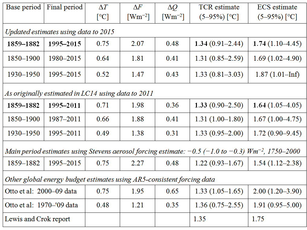
Table 1: TCR and ECS estimates (medians and 5-95% uncertainty ranges) on various bases. Main results are shown in bold. ΔT, ΔF and ΔQ are changes between base and final period mean values.

The consistency of the TCR estimates across periods is supportive of the accuracy of the energy budget estimation method, although with only four more year’s data being added one would not expect a large change in TCR estimates. Whilst four years is far too short a period to estimate TCR or (even more so) ECS over, it is interesting to note that TCR estimated from ΔT and ΔF from 1859– 82 to 2012–15, the added years, is almost the same as for the full 1995–2015 period, at 1.30°C.

Although the AR5 allowance for an upwards trend in >2000 m deep OHC from 1992 on has been retained, a post-AR5 study indicates that, contrary to the studies relied upon in AR5, >2000 m OHC has been reducing rather than increasing since 1992.[10] If the AR5 based allowance for warming in the deep ocean were omitted, the preferred ECS estimate based on 1859-1882 to 1995-2015 changes would reduce from 1.74°C to 1.68°C.

Now that the Argo network has had reasonable coverage down to a depth of ~2000 m for a decade, it is practicable to estimate ECS using Argo-period-only OHC data, although a decade is on the short side for reliable estimation. I have done so using a final period of 2006-2015, substituting the trend in annual mean NOAA/Levitus 0-2000 m OHC data for the mixture of Argo and pre-Argo, pentadal and annual, OHC data that has to be used for the 1995-2015 period. An allowance for OHC increases below 2000 m was again added, giving a planetary heat uptake of 0.78 Wm⁻². The resulting TCR estimate is 1.32°C, and 1.84°C for ECS. However, there are reasons for thinking that the NOAA/Levitus mapping (infilling) method may lead to an overestimation of the increase in OHC as observational coverage increases, which it did over 2006–2015 as the recently-established Argo network became denser. The Lyman and Johnson 0-1800 m OHC Argo dataset,[11] which uses a mapping method that largely avoids such a bias, produces an OHC trend over 2006-2011 0.07 Wm⁻² below that per the NOAA/Levitus data, after allowing for heating in the 1800-2000 m layer. Unfortunately, the Lyman and Johnson data ends in 2011, but if the NOAA/Levitus dataset had overestimated the ocean heating rate by 0.07 Wm⁻² throughout 2006-2015, the 1.84°C ECS estimate would reduce to 1.76°C. Another estimate for the 0-2000 m Argo-only OHC trend increase is 0.44Wm⁻² over 2006-2013,[12] which is likewise 0.07 Wm⁻² smaller than the NOAA/Levitus estimate for the same period, again suggesting an ECS estimate of 1.76°C.

Appraising claims that energy budget studies underestimate equilibrium climate sensitivity

It has been claimed (apparently based on HadCRUT4v1) that incomplete coverage of high-latitude zones in the HadCRUT4 dataset biases down its estimate of recent rates of increase in GMST.[13] Representation in the Arctic has improved in subsequent versions of HadCRUT4. Even for HAdCRUT4v2, used in LC14, the increase in GMST over the period concerned actually exceeds the area-weighted average of increases for ten separate latitude zones, so underweighting of high-latitude zones does not seem to cause a downwards bias. The issue appears to relate more to interpolation over sea ice than to coverage over land and open ocean in high latitudes. The possibility of coverage bias in HadCRUT4 has since been independently examined by ECMWF using their well-regarded ERA interim reanalysis dataset. They found no reduction in that dataset’s 1979-2014 trend in 2 m near-surface air temperature when the globally-complete coverage was reduced to match that of HadCRUT4v4.[14] Since the ERA interim reanalysis combines observations from multiple sources and of multiple atmospheric variables, based on a model that is well-proven for weather forecasting, it should in principle provide a more reliable infilling of areas where surface data is very sparse, such as high-latitude zones, than mechanistic methods such as kriging. Moreover, during the early decades of the HadCRUT4 record (which includes the 1859-1882 base period) data was sparse over much of the globe, and infilling may introduce significant errors. It has also been claimed, based on climate model simulations, that the use of sea surface temperature (SST) as a proxy for near-surface air temperature for ocean areas causes a downward bias.[15] There are some theoretical grounds supporting this argument. However, the two main surface temperature datasets that are based (on a decadal timescale upwards) on air temperature above the ocean as well as land, and which moreover interpolate to obtain complete or near complete global coverage (NOAAv4.01 and GISSTEMP) show an almost identical change in mean GMST to that per HadCRUT4v4 from 1880-1899, the first two decades they cover, to 1995-2015, the final period used for this update of LC14. Whilst some downwards bias in HadCRUT4v4 may nevertheless exist, there are also possible sources of upwards bias, such as urbanisation effects.

It has also been claimed that a downward bias in TCR,[16] and also ECS,[17] estimation from historical data arises from other types of forcing having different effects on GMST than does CO₂ (that is, having efficacies differing from one). Spatially inhomogeneous forcing, principally from aerosols, has been raised as a particular concern, with a levelling off of aerosol forcing in recent decades adding to potential underestimation. However, these model-based results are contradicted by other model-based studies that use simulations specifically designed for measuring forcing efficacies. The first and most thorough investigation of forcing efficacies was by Hansen et al.[18] They found almost all types of forcing to have efficacies very close to one provided that they were measured by ERF, with volcanic and ozone forcing having efficacies slightly below one and methane forcing having an efficacy slightly above one. Moreover, they found that the historical mix of forcings over 1880–2000 had an ERF efficacy of almost exactly one. Marvel et al. (2016)¹⁷ also found aerosol ERF to have an efficacy extremely close to one, and although it found ozone RF and ERF to have an efficacies well below one, that appears to have been due to an inappropriate climate state being used to measure ozone forcing, resulting in it being substantially overestimated.[19] Other studies also find no evidence for aerosol ERF having a high efficacy.[20] There is, however, evidence that volcanic forcing (which had a zero trend over the 1880-2000 period investigated by Hansen et al.) has a low efficacy, particularly when measured by RF.[21] This finding does not affect LC14 or the update thereof given here, since the base and final periods have been matched as to their levels of volcanic forcing. To summarize, there are no good grounds for believing that the LC14 original or updated results are biased by historical forcings having different efficacies to that of CO₂.

Strictly, ECS estimated from transient climate change, as here, represents effective rather than equilibrium climate sensitivity, as the ocean has not reached equilibrium. In many current generation (CMIP5) atmosphere-ocean general circulation models (AOGCMs), equilibrium climate sensitivity exceeds effective sensitivity derived from forcing with a time-profile comparable to that available from the instrumental record. From analysing all CMIP5 models for which I have data, the mean difference in the two ECS measures is somewhat under 10%, using the same standard method of estimating AOGCM equilibrium sensitivity as in IPCC AR5. It is unknown whether or to what extent the two measures differ in the real world. Paleoclimate ECS estimates based on the transition from the last glacial maximum to the Holocene (LGM studies), may cast some light on this, despite considerable uncertainties, although estimates of ECS from more distant paleoclimate periods are difficult to directly compare with ECS in today’s climate state.[22] Simple calculations in which GMST at the LGM is divided by the total estimated forcing, both relative to the preindustrial state, have long been used to generate estimates of equilibrium climate sensitivity.[23] Current best estimates of GMST (4.0 ± 0.8°C below preindustrial)[24] and of relevant forcings (6–11 Wm⁻² below preindustrial)[25] at the LGM imply an ECS estimate of 1.75°C, essentially identical to the updated instrumental-observation energy budget estimate presented here. That suggests effective and equilibrium climate sensitivities in the real world may be very close to each other, but only about half the average equilibrium sensitivity of CMIP5 models.

Conclusions

Estimation of TCR seems remarkably robust to the analysis period, although the concentration of TCR best estimates in the narrow 1.31–1.36°C band may be fortuitous. However, estimating TCR by regressing GMST on total forcing with years affected by volcanic activity excluded, as in Gregory and Forster (2008),[26] produces reasonably consistent values over different long periods: 1.38°C over the full 1850–2015 HadCRUT4 period; 1.41°C over 1945–2015 (a period with zero trend in volcanic forcing that approximately spans the 65-70 year apparent periodicity of the AMO); and 1.27°C over 1850–1965, a period with a modest trend in volcanic activity (1.32°C when scaling volcanic forcing by an efficacy factor of 0.55, found in LC14 to be appropriate). To the extent that the forcing and GMST estimates used are in error, all these TCR best estimates would of course change. The dominant source of uncertainty is the AR5 aerosol forcing estimate.

ECS estimates are somewhat more sensitive to the period and the particular OHC dataset used, and the lack of OHC measurements prior to the 1950s makes dependence on model-based OHC estimates for the base period difficult to avoid. Based on the latest version of the HadCRUT4 dataset, an early base period and longer than decadal final period, the ECS best estimates fall in the range 1.65–1.75°C depending on the final period and OHC dataset used. For two base period – final period combinations not meeting these criteria, the ECS best estimates are around 1.85°C, but these are likely less reliable. There are some grounds for thinking that the final period OHC increases used may be slightly overestimated, at least in some cases. The uncertainty in ECS estimates remains very large. As for TCR, this is due primarily to uncertainty in the AR5 aerosol forcing estimate.

If the aerosol best estimates and uncertainty range are derived from Stevens (2015) rather than AR5, the best estimates for TCR and ECS reduce by respectively slightly less and slightly more than 10%, but the upper 95% bounds are greatly reduced: from 2.44°C to 1.67°C for TCR and from 4.45°C to 2.38°C for ECS. This highlights the importance of narrowing uncertainty regarding aerosol forcing.

There appears to be little substance in claims that global energy budget studies systematically underestimate TCR and/or ECS to a significant extent, although the possibility of a modest degree of underestimation cannot be ruled out.

Appendix A – derivation of individual forcings for 2012 to 2015

Well mixed greenhouse gases

Forcing from CO₂, CH₄ and N₂O was calculated for each year from 2011 to 2015 using data for mean atmospheric concentrations[27] and the formulae in AR5 8.SM.3. Forcing from minor GHGs was projected based on the recent growth rates and levels of forcing by CFCs, HCFCs and HFCs shown in AR5 Figure 8.6. I estimate that these imply a growth rate of 0.02 Wm⁻²decade⁻¹, in line with the growth rate implied by the difference between the 2005 and 2011 Total halogens forcing values in AR5 Table 8.2. The annual change from 2011 in the thus calculated total forcing from GHG was then added to the AR5 GHG forcing estimate of 2.83 Wm⁻² (which uses marginally different concentrations of CO₂, CH₄ and N₂O). This results in the 2015 GHG forcing value being 2.98 Wm⁻², of which CO₂ accounts for 1.94 Wm⁻².

Aerosols

AR5 estimates that total aerosol forcing declined at a rate of 0.24% per annum over 2002-11. Global aerosol optical depth (AOD) estimates over 2014–12 from three satellite instrumentation based datasets and a specialised model driven by assimilated meteorological observations are very similar, with three having trends indistinguishable from zero and one a trend of approximately −1% per annum, all with no sign of any change in trend (Ma and Yu 2015, Figure 1.a).[28] Consistent with this, the AR5 estimates are extrapolated from −0.90 Wm⁻² in 2011 to 2012-15 using the same −0.24% per annum trend as over 2002-11, reaching −0.891 Wm⁻² in 2015.

Ozone

AR5 presents evidence for both tropospheric and stratospheric ozone concentrations gradually increasing since the late 20th century, resulting in positive forcing trends. I am not aware of any evidence that these trends have changed materially since 2011. Therefore, I extrapolate the AR5 2011 tropospheric and stratospheric ozone forcing values using their respective trends over the decade to 2011. The change by 2015 is an increase of 0.007 Wm⁻². Satellite observations suggest that the post 2011 increase in stratospheric ozone forcing has been rather faster than per the trend over the previous decade,[29] but the difference in forcing is only 0.004 W m⁻² by 2015 and the data are noisy so the trend increase has been used.

Other anthropogenic forcings

The AR5 estimates for minor land use change (albedo), stratospheric water vapour, black carbon on snow and contrails forcings have likewise been extrapolated from 2011 to 2015 using their trends over the decade to 2011. The net effect is an increase in forcing of 0.008 Wm⁻² by 2015.

Solar

I updated solar forcing using TSI data from SORCE,[30] rebasing it to give the same anomaly, 0.03 Wm⁻² , in 2011 as per AR5. Solar forcing climbs over 2012-15, reaching 0.119 Wm⁻² in 2015.

Volcanic

The post 1850 AR5 volcanic forcing estimates are slightly rounded from −25x stratospheric AOD, based on the Sato dataset.[31] The latest value in that dataset is for 2012, and implies a slightly smaller forcing of −0.107 Wm⁻² in 2012, very close to the AR5 2006–11 mean, than in 2011, which was more affected by the Nabro eruption. Sulphur dioxide emissions from explosive volcanic eruptions during 2013 to 2015 and the resulting stratospheric AOD levels remained at a similarly modest level to 2012 (Carn et al. 2016, Figure 9).[32] I have therefore taken volcanic forcing to be −0.107 Wm⁻² throughout 2012-15.

Appendix B – estimation of heat uptake rate

LC14, following Otto et al. (2013), used the difference between the OHC estimates for the first and last years when calculating planetary heat uptake for the final period. With the final year OHC no longer representing an average over several years, it is more appropriate to estimate heat uptake using the linear trend over the period rather than the differencing method. The 1995-2015 heat uptake rate is 0.63 Wm^−1, whether calculated using the newly adopted linear trend method or the previous differencing method.

Since error standard deviation estimates are available for all years of OHC data, uncertainty in the regression slope is estimated by performing a large ensemble of regressions each with all individual year heat content values perturbed by random draws from their uncertainty distributions. To allow for non-independence of errors in nearby years, which is to be expected even when 3 or 5 year running means are not used, all estimated heat content uncertainties are multiplied by sqrt(3). This multiplier reflects the dominance of uncertainty in 3-year mean 0–700 m OHC until the mid 2000s. Its use results in a slightly lower standard error estimate for the 1995-2011 heat uptake rate, of 0.081 Wm⁻², that the 0.087 Wm⁻² when using the difference method. That is consistent with use of regression producing only a modest reduction in uncertainty for estimating heat uptake over fifteen years when the initial and final values used in the difference method are dominated by means over several years.

The scaled-down model-derived estimates of heat uptake in the base periods, and uncertainty therein, are unchanged from LC14.

Nicholas Lewis

[1] Lewis N., Curry J.A., 2014: The implications for climate sensitivity of AR5 forcing and heat uptake estimates. Clim Dyn, 45, 1009-1023. Final accepted version available here

[2] In addition, AR5 estimates black carbon deposited on snow to have 2–4 times an effect on GMST per unit forcing, compared to other types of forcing. This was taken account of in LC14. For volcanic forcing, it is not apparent that AR5 considered the relationship between RF and ERF.

[3] Data available here

[4] Available at http://www.nodc.noaa.gov/OC5/3M_HEAT_CONTENT/basin_avt_data.html

[5] Available at http://www.data.jma.go.jp/gmd/kaiyou/english/ohc/ohc_global_en.html

[6] TCR and ECS estimates are almost identical whether using a 1987-2015 or a 1980-2015 final period, with a 1850-1900 base period

[7] Stevens, B (2015) Rethinking the lower bound on aerosol radiative forcing. J Clim, 28, 4794–4819. Details of the derivation from that paper of a best estimate time series for aerosol forcing are available here.

[8] Otto A et al (2013). Energy budget constraints on climate response. Nat Geosci 6:415–416

[9] Lewis N and M Crok (2014): A Sensitive Matter. Published by the Global Warming Policy Foundation, London. 65 pp

[10] Liang, X, C Wunsch, P Heimbach and G Forget (2015). Vertical Redistribution of Oceanic Heat Content. J Clim, 28, 3821-3833

[11] Lyman J, G Gregory (2014). Estimating Global Ocean Heat Content Changes in the Upper 1800m since 1950 and the Influence of Climatology Choice. J Clim, 27, 1945-1957. The omission of OHC changes in the 1800-2000 m layer is estimated to account for no more than a heating rate of 0.02 W/m² over 2006-2011.

[12] Roemmich, D. et al. (2015) Unabated planetary warming and its anatomy since 2006. Nature Clim. Change 5, 240–245. The 0.44 W m⁻² value is based on the average of the OI and RSOI Global values in Table 1, with 0.1 added to the OI value to allow for its smaller spatial domain, then divided by 0.83 to allow for the areas not sampled, and converted from 10²¹ J yr⁻¹ to W m⁻².

[13] Cowtan, K. & Way, R. G. (2014) Coverage bias in the HadCRUT4 temperature series and its impact on recent temperature trends. Q. J. R. Meteorol. Soc. 140, 1935_1944.

[14] See http://www.ecmwf.int/en/about/media-centre/news/2015/ecmwf-releases-global-reanalysis-data-2014-0. The data graphed in the final figure shows the same 1979-2014 trend whether or not coverage is reduced to match HadCRUT4.

[15] Cowtan, K et al. (2015) Robust comparison of climate models with observations using blended land air and ocean sea surface temperatures. Geophys. Res. Lett., 42, 6526–6534.

[16] Shindell, DT (2014) Inhomogeneous forcing and transient climate sensitivity. Nat Clim Chg, 4, 274–277

[17] Marvel, K, et al. (2015) Implications for climate sensitivity from the response to individual forcings. Nat Clim Chg DOI: 10.1038/NCLIMATE2888

[18] Hansen J et al (2005) Efficacy of climate forcings. J Geophys Res, 110: D18104, doi:101029/2005JD005776

[19] See http://climateaudit.org/2016/01/08/appraising-marvel-et-al-implications-of-forcing-efficacies-for-climate-sensitivity-estimates/

[20] Ocko IB, V Ramaswamy and Y Ming (2014) Contrasting climate responses to the scattering and absorbing features of anthropogenic aerosol forcings. J. Climate, 27, 5329–5345; Forster, P (2016) Inference of Climate Sensitivity from Analysis of Earth’s Energy Budget. Annu. Rev. Earth Planet. Sci. 2016. 44, doi: 10.1146/annurev-earth-060614-105156

[21] Gregory, J M et al. (2016) Small global-mean cooling due to volcanic radiative forcing. Clim Dyn DOI 10.1007/s00382-016-3055-1. See also the discussion of volcanic forcing in LC14.

[22] Section 10.8.2.4 of AR5

[23] See, e.g., Annan, J and Hargreaves, J., 2015. A perspective on model-data surface temperature comparison at the Last Glacial Maximum. Quaternary Science Reviews, 107, 1-10

[24] Annan, J.D., Hargreaves, J.C., 2013. A new global reconstruction of temperature changes at the Last Glacial maximum. Clim. Past 9 (1), 367-376.

[25] Annan, J.D., Hargreaves, J.C., 2006. Using multiple observationally-based constraints to estimate climate sensitivity. Geophys. Res. Lett. 33, L06704.

[26] Gregory JM, Forster PM (2008) Transient climate response estimated from radiative forcing and observed temperature change. J Geophys Res 113:D23105. Halving their volcanic forcing threshold, to −0.25 Wm⁻², has a negligible effect on TCR estimates.

[27] Concentrations up to 2014 from http://ds.data.jma.go.jp/gmd/wdcgg/pub/global/globalmean.html. Increase from 2014 to 2015 was based: for CO₂, on the Mauna Loa mean from ftp://aftp.cmdl.noaa.gov/products/trends/co2/co2_annmean_mlo.txt; for CH₄, on the smoothed trend curve at http://www.esrl.noaa.gov/gmd/ccgg/trends_ch4/; and for N₂O on data at ftp://ftp.cmdl.noaa.gov/hats/n2o/combined/HATS_global_N2O.txt

[28] X Ma and F Yu (2015): Seasonal and spatial variations of global aerosol optical depth: multi-year modelling with GEOS-Chem-APM and comparisons with multiple-platform observations. Tellus B 2015, 67, 25115. http://www.tellusb.net/index.php/tellusb/article/view/25115

[29] KNMI MSR ozone data at http://www.temis.nl/protocols/o3field/o3mean_msr.php shows a global increase of 4.3 Dobson units for 2015 over the mean for 2008-11, and regressing AR5 stratospheric O₃ forcing on the MSR data yields a slope of 0.0016 Wm⁻² Dobson unit⁻¹ (correlation: 0.80), implying 2015 forcing of −0.044 Wm⁻² vs −0.048 Wm⁻² from continuing the 2001-11 trend.

[30] Downloaded from http://lasp.colorado.edu/lisird/sorce/sorce_tsi/index.html; divided by 4 to give mean TOA downward solar radiation

[31] http://data.giss.nasa.gov/modelforce/strataer/tau.line_2012.12.txt

[32] Carn S.A., L. Clarisse, A.J. Prata (2016) Multi-decadal satellite measurements of global volcanic degassing. Jnl of Volcanology and Geothermal Research 311, 99–134